

Category: News
GPO – MSI Application Deployment File Share Permissions
Hello-
How can I configure permissions on my MSI application deployment share so that I can deploy applications via GPO, but also deny users any access to the MFT files (or the entire share). There is sensitive information in these MFT files, and I don’t want end users to access them. I know could hide$ the share, but I’d prefer to lock it down if possible.
Thank you!
Hello- How can I configure permissions on my MSI application deployment share so that I can deploy applications via GPO, but also deny users any access to the MFT files (or the entire share). There is sensitive information in these MFT files, and I don’t want end users to access them. I know could hide$ the share, but I’d prefer to lock it down if possible. Thank you! Read More

Planner: Copy a plan to a premium plan
When you use the trial feature for premium plans you can promote a plan to be a premium plan a.k.a. Project for the web project, to get the additional features of timelines, goals, Copilot and more! This feature will also be coming to new Planner for all basic plans, but probably not until the summer 2024. For now, there is a work around using a specific Url with the Plan ID of the basic plan added – then the magic happens, and you get a premium plan (some limitations apply – see the docs linked below).
A basic Planner plan you a board view and a grid view, and some charts, but if you need more then time to look at making a premium plan from it.
A basic Planner plan
The workaround until the in-app feature becomes available is to craft a Url that starts with your Project for the web Url, including locale and tenant, adds some specific parameters and adds on the plan id. It will look something like this:
https://project.microsoft.com/<your tenant name>.onmicrosoft.com/en-US#/hubnew?importPlanId=<your Plan ID>
Hopefully you know your tenant name, or just navigate to project.microsoft.com and it should complete the Url up to the locale part (en-US in the able example) once you have signed in. To this you add the #/hubnew?importPlanId= part and then the plan id. It isn’t easy to find the plan id in Teams (but if you know your way around F12 Dev Tools you can find it) but easier to just look for your plan at tasks.office.com and open it – then the Url will contain your plan id. In my case the Url in Planner is:
https://tasks.office.com/brismith.onmicrosoft.com/en-US/Home/Planner/#/plantaskboard?groupId=d132c3ce-e77b-7bfc-a703-3aceaed05a37&planId=q_E7IvbSGkCD1f537UPBUGUADys7
and the final part is the plan id – after planId= – so q_E7IvbSGkCD1f537UPBUGUADys7
Adding this to the project Url and the parameter part gives me a full Url of:
https://project.microsoft.com/brismith.onmicrosoft.com/en-US#/hubnew?importPlanId=q_E7IvbSGkCD1f537UPBUGUADys7
Once I have this, I can paste it into my browser, log in if I don’t already have an active session, then the magic starts!
After a short while you will see this screen briefly:
then you will see the background change to your new premium plan and the dialog changes to:
Be sure to review the document – the “Learn more” link goes to this article https://prod.support.services.microsoft.com/en-us/office/import-a-plan-into-a-project-for-the-web-016f9e4d-28c6-4f61-a1b1-82187185977d and probably the most important section relates to the task limits. Only 950 tasks will be imported into your premium plan. See the other sections too to be sure you get what you need:
But that’s it. Hopefully that will help until the UI has an option to import basic Planner plans to the premium experience so you can then use all of the extra features of premium plans:
and use it in new Planner too – under My Plans:
Any questions – add them below and I’ll get back to you.
Microsoft Tech Community – Latest Blogs –Read More

New Blog | Navigating New Application Security Challenges Posed By GenAI
By Asaf Harari
GenAI applications—software powered by large language models (LLMs) are changing the way we interact with digital platforms. These advanced applications are designed to understand, interpret, and generate human-like text, code and various forms of media, making our digital experiences more seamless and personalized than ever before. With the increasing availability of LLMs, we can expect to see even more innovative applications of this technology in the future. However, it is important to carefully consider the potential security challenges related to GenAI applications and the underline LLM.
While security challenges in machine learning models have been studied for some time, such as the potential for adversarial attacks where input data can be manipulated to mislead the model. However, challenges specific to LLMs are still relatively unexplored and pose a blind spot for researchers and practitioners. LLMs are distinct from other software tools and machine learning elements in terms of their functionality, the way GenAI applications employ them, and the way users engage with them. For these reasons, for the development and use of GenAI applications, it’s crucial to implement GenAI security best practices, Zero Trust architecture, posture management solutions, and conduct red team exercises. Microsoft is at the forefront of not only deploying GenAI applications but also ensuring the security of these applications, their related data, and their users.
In this blog post, we will review the unique cybersecurity challenges that GenAI apps and the underline LLMs pose according to their special behavior, their unique use, and their interaction with the users.
Read the full post here: Navigating New Application Security Challenges Posed By GenAI

Adding a field parameter fields to TopN visual filter pane
I have created a field parameter table as below:
I have used above field parameter in below visual x-axis:
Now its working well! But I want to filter this visual for TopN values as shown below based on parameter table fields column as shown below:
But when i drag this field parameter column in filter this visual pane ‘By value’ it shows First Parameter and it doesn’t aggregate.
I am confused how to filter visual by the top 20 ‘Name’ column by variance Field parameter fields column.
Can you please help us with this?
PFA file here Portfolio Performance – v2.12 – Copy.pbix
Thanks in advance!
Hi @Sergei Baklan I have created a field parameter table as below: I have used above field parameter in below visual x-axis: Now its working well! But I want to filter this visual for TopN values as shown below based on parameter table fields column as shown below: But when i drag this field parameter column in filter this visual pane ‘By value’ it shows First Parameter and it doesn’t aggregate.I am confused how to filter visual by the top 20 ‘Name’ column by variance Field parameter fields column. Can you please help us with this? PFA file here Portfolio Performance – v2.12 – Copy.pbix Thanks in advance! Read More
LSASS Memory Dump Handle Access – poqexec.exe ?
We are seeing SIEM alerts for LSASS Memory Dump Handle Access for the ‘C:WindowsSystem32poqexec.exe’ process (Primitive Operations Queue Executor) on several endpoints with the computer account name.
However, Defender for Endpoint is not picking this up as an alert, nor is the process listed in the device’s timeline.
We are seeing SIEM alerts for LSASS Memory Dump Handle Access for the ‘C:WindowsSystem32poqexec.exe’ process (Primitive Operations Queue Executor) on several endpoints with the computer account name. However, Defender for Endpoint is not picking this up as an alert, nor is the process listed in the device’s timeline.I am not finding much online about poqexec.exe and possible interaction with LSASS and I was hoping to get some insight here.Anyone see this before and can help me validate the behavior? Event/log details:message: “A handle to an object was requested.Subject:Security ID: S-1-5-18Account Name: <computerAccount$>Account Domain: <ourDomain>Object:Object Server: SecurityObject Type: FileObject Name: C:WindowsSystem32lsass.exeHandle ID: 0x70Resource Attributes: -Process Information:Process ID: 0x6fcProcess Name: C:WindowsSystem32poqexec.exeAccess Request Information:Transaction ID: {2801ddbe-0b5e-11ef-9edb-4c3488257915}Accesses: DELETEREAD_CONTROLWRITE_DACWRITE_OWNERSYNCHRONIZEReadData (or ListDirectory)ReadEAReadAttributesWriteAttributesAccess Reasons: -Access Mask: 0x1F0189Privileges Used for Access Check: SeBackupPrivilegeSeRestorePrivilegeRestricted SID Count: 0” Read More
REGISTER TODAY: Monthly Azure Nonprofit Office Hours | May – June
Hello Partners,
If you missed our April Azure Office Hours, view the sessions on-demand:
April 2024 Nonprofit Open Azure Office Hours | Watch Now
Join us for these upcoming sessions!
May 29, 2024
8:00am – 9:00am PST | Register Here
4:00pm – 5:00pm PST | Register Here
June 20, 2024
8:00am – 9:00am PST | Register Here
4:00pm – 5:00pm PST | Register Here
Please come prepared with questions!
Hello Partners,
If you missed our April Azure Office Hours, view the sessions on-demand:
April 2024 Nonprofit Open Azure Office Hours | Watch Now
Join us for these upcoming sessions!
May 29, 2024
8:00am – 9:00am PST | Register Here
4:00pm – 5:00pm PST | Register Here
June 20, 2024
8:00am – 9:00am PST | Register Here
4:00pm – 5:00pm PST | Register Here
Please come prepared with questions! Read More
What did you learn at Impact Summit in NYC? Explore – Adapt – Adopt!
On May 8, nonprofit innovators gathered in NYC to learn about transformation across the nonprofit world – and how tools like AI can support growth and capacity.
If you attended the session “Redefining productivity for nonprofits with AI” with Devi Thomas and Brandonlon Bartlett, tell what you thought! What takeaways and insights did you get from the table discussions based on the Explore-Adapt-Adopt frameworks?
Watch for the virtual Impact Summit coming on May 15 – and keep the conversation going here!
On May 8, nonprofit innovators gathered in NYC to learn about transformation across the nonprofit world – and how tools like AI can support growth and capacity.
If you attended the session “Redefining productivity for nonprofits with AI” with Devi Thomas and Brandonlon Bartlett, tell what you thought! What takeaways and insights did you get from the table discussions based on the Explore-Adapt-Adopt frameworks?
Watch for the virtual Impact Summit coming on May 15 – and keep the conversation going here! Read More
Each desktop needs it’s own taskbar
I am dumbfounded about why you can have multiple desktops but only one taskbar? It makes it pointless in my view.
Please at least ensure that only windows opened from a particular desktop are shown in the taskbar for that desktop. But a completely customized taskbar per desktop would be even better.
I am dumbfounded about why you can have multiple desktops but only one taskbar? It makes it pointless in my view. Please at least ensure that only windows opened from a particular desktop are shown in the taskbar for that desktop. But a completely customized taskbar per desktop would be even better. Read More
Defender Firewall rules – Event ID 2001
In my organization, we’re moving away from Trellix suite to MDE. All of my policies (DLP, AV, Exclusions, etc…) are working, but not the Firewall general settings nor the Firewall Rules. Defender portal indicates that the Firewall settings policy was successful, but the rules are not. Our workstations are hybrid-joined, but managed by SCCM/MDE. When I look at the Event View for SENSE (channel Microsoft-Windows-SENSE/Operational) related events, I get an event ID 2001, and the info is: SenseCM: WRN: FW VA: no rule TESTING POLICY
The rule TESTING POLICY exists in my Defender portal, under Endpoint security policies, so it seems like my test workstation can see that policy, but it doesn’t get applied, and also the Firewall settings don’t get applied, as it doesn’t appear to change the default block/allow for Outbound or Inbound for each of the Firewall profile (Public, Private, Domain).
Anything suggestion will be appreciated.
In my organization, we’re moving away from Trellix suite to MDE. All of my policies (DLP, AV, Exclusions, etc…) are working, but not the Firewall general settings nor the Firewall Rules. Defender portal indicates that the Firewall settings policy was successful, but the rules are not. Our workstations are hybrid-joined, but managed by SCCM/MDE. When I look at the Event View for SENSE (channel Microsoft-Windows-SENSE/Operational) related events, I get an event ID 2001, and the info is: SenseCM: WRN: FW VA: no rule TESTING POLICY The rule TESTING POLICY exists in my Defender portal, under Endpoint security policies, so it seems like my test workstation can see that policy, but it doesn’t get applied, and also the Firewall settings don’t get applied, as it doesn’t appear to change the default block/allow for Outbound or Inbound for each of the Firewall profile (Public, Private, Domain). Anything suggestion will be appreciated. Read More
Partner Blog | How Microsoft Copilot and ServiceNow Now Assist enhance employee & IT admin choice
As Microsoft works to enable AI at the enterprise level, our focus is on building sophisticated productivity tools that integrate with our ecosystem of partners. For example, during last year’s Microsoft Ignite conference, we provided an early preview of how ServiceNow’s integration with Microsoft Copilot would bring generative AI capabilities to IT and employee experiences. I recently had the pleasure of joining ServiceNow’s President and Chief Operating Officer CJ Desai on stage at the company’s marquee event, Knowledge 2024 in Las Vegas, to unveil three compelling scenarios that fulfill the promise of Copilot and Now Assist, ServiceNow’s generative AI experience.
Now Assist AI delivers direct, relevant, and conversational responses to employee requests, and connects exchanges to AI-powered workflows on ServiceNow’s platform to take actions on behalf of the employee. I’ll share more on how we’ve integrated Copilot and Now Assist to supercharge the workforce using the scenarios from Knowledge 2024, but first let’s discuss the extensibility model used by ServiceNow for the integration.
There are various ways to extend Copilot, which provide the starting point for partners looking to harness AI and bring Copilot capabilities to your apps. We are also working on a new approach to extensibility that makes it possible for independent software vendors (ISVs) to bring their own generative AI technologies into Copilot experiences and hand off users to their own third-party copilots, ensuring user experiences and workflows are streamlined. ServiceNow is taking advantage of this new option by allowing users to execute ServiceNow workflows via Now Assist to improve employee productivity and deliver an improved experience.
Continue reading here
Microsoft Tech Community – Latest Blogs –Read More
Single-region deployment using Secure Virtual WAN Hub with Routing-Intent and Global Reach
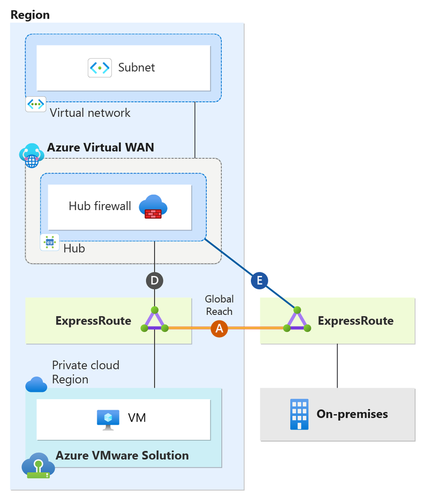
This article describes the best practices for connectivity, traffic flows, and high availability of single-region Azure VMware Solution when using Azure Secure Virtual WAN with Routing Intent. You will learn the design details of using Secure Virtual WAN with Routing-Intent, when using Global Reach. This article breaks down Virtual WAN with Routing Intent topology from the perspective of an Azure VMware Solution private cloud, on-premises sites, and Azure native. The implementation and configuration of Secure Virtual WAN with Routing Intent are beyond the scope and aren’t discussed in this document.
Secure Virtual WAN with Routing Intent is only supported with Virtual WAN Standard SKU. Secure Virtual WAN with Routing Intent provides the capability to send all Internet traffic and Private network traffic to a security solution like Azure Firewall, a third-party Network Virtual Appliance (NVA), or SaaS solution. In the scenario, we have a single region network. There’s a Virtual WAN with one hub. The hub has an Azure Firewall deployed, essentially making it a Secure Virtual WAN hub. Having a Secure Virtual WAN hub is a technical prerequisite to Routing Intent. The Secure Virtual WAN hub has Routing Intent enabled.
Note
When configuring Azure VMware Solution with Secure Virtual WAN Hubs, ensure optimal routing results on the hub by setting the Hub Routing Preference option to “AS Path.” – see Virtual hub routing preference
The single region consists of its own Azure VMware Solution Private Cloud and an Azure Virtual Network. Additionally, there’s an on-premises site connecting back to the hub. Furthermore, Global Reach connectivity exists within the environment. Global Reach establishes a direct logical link via the Microsoft backbone, connecting Azure VMware Solution to on-premises. As shown in the diagram, Global Reach connections don’t transit the Hub firewall. So, Global Reach traffic between on-premises and Azure VMware Solution, and vice versa, remains uninspected.
Note
When utilizing Global Reach, consider enhancing security between Global Reach sites by inspecting traffic within the Azure VMware Solution environment’s NSX-T or an on-premises firewall.
Understanding Topology Connectivity
Connection
Description
Connections (D)
Azure VMware Solution private cloud managed ExpressRoute connection to the hub.
Connection (A)
Azure VMware Solution Global Reach connection back to on-premises.
Connections (E)
on-premises ExpressRoute connection to the hub.
The following sections cover traffic flows and connectivity for Azure VMware Solution, on-premises, Azure Virtual Networks, and the Internet.
This section focuses only on the Azure VMware Solution Cloud’s perspective. Azure VMware Solution private cloud has an ExpressRoute connection to its hub (connection labeled as “D”).
The Azure VMware Solution Cloud Region establishes a connection to on-premises via ExpressRoute Global Reach, depicted as Global Reach (A) in the diagram. It’s important to note that traffic via Global Reach doesn’t transit the Hub firewall.
Ensure that you explicitly configure Global Reach (A). It’s imperative to do this step to prevent connectivity issues between on-premises and Azure VMware Solution. For more information, see traffic flow section.
The diagram illustrates traffic flows from the perspective of the Azure VMware Solution Private Cloud.
Traffic Flow Chart
Traffic Flow Number
Source
Direction
Destination
Traffic Inspected on Secure Virtual WAN Hub firewall?
1
Azure VMware Solution Cloud
→
Virtual Network
Yes, traffic is inspected at the Hub firewall
2
Azure VMware Solution Cloud
→
on-premises
No, traffic bypasses firewall and transits Global Reach (A)
This section focuses only on the on-premises site. As shown in the diagram, the on-premises site has an ExpressRoute connection to the hub (connections labeled as “E”). On-premises systems can communicate to Azure VMware Solution via connection Global Reach (A).
Ensure that you explicitly configure Global Reach (A). It’s imperative to do this step to prevent connectivity issues between on-premises and Azure VMware Solution. For more information, see traffic flow section.
The diagram illustrates traffic flows from an on-premises perspective.
Traffic Flow Chart
Traffic Flow Number
Source
Direction
Destination
Traffic Inspected on Secure Virtual WAN Hub firewall?
3
on-premises
→
Azure VMware Solution Cloud
No, traffic bypasses firewall and transits Global Reach (A)
4
on-premises
→
Virtual Network
Yes, traffic is inspected at the Hub firewall
This section focuses only on connectivity from the Azure Virtual Network perspective. As depicted in the diagram, the Virtual Network is peering directly to the hub.
A Secure Hub with enabled Routing Intent always sends the default RFC 1918 addresses (10.0.0.0/8, 172.16.0.0/12, 192.168.0.0/16) to peered Virtual Networks, plus any other prefixes that are added as “Private Traffic Prefixes” – see Routing Intent Private Address Prefixes. In our scenario, with Routing Intent enabled, all resources in the Virtual Network currently possess the default RFC 1918 addresses and use the Hub firewall as the next hop. All traffic ingressing and egressing the Virtual Network will always transit the Hub firewall. For more information, see traffic flow section.
Traffic Flow Chart
Traffic Flow Number
Source
Direction
Destination
Traffic Inspected on Secure Virtual WAN hub firewall?
5
Virtual Network
→
Azure VMware Solution Cloud
Yes, traffic is inspected at the Hub firewall
6
Virtual Network
→
Azure VMware Solution Cloud
Yes, traffic is inspected at the Hub firewall
This section focuses only on how internet connectivity is provided for Azure native resources in the Virtual Network and the Azure VMware Solution Private Cloud. There are several options to provide internet connectivity to Azure VMware Solution. – see Internet Access Concepts for Azure VMware Solution
Option 1: Internet Service hosted in Azure
Option 2: VMware Solution Managed SNAT
Option 3: Azure Public IPv4 address to NSX-T Data Center Edge
Although you can use all three options with Single Region Secure Virtual WAN with Routing Intent, “Option 1: Internet Service hosted in Azure” is the best option when using Secure Virtual WAN with Routing Intent and is the option that is used to provide internet connectivity in the scenario. The reason why “Option 1” is considered the best option with Secure Virtual WAN is due to its ease of security inspection, deployment, and manageability.
With Routing Intent, you can choose to generate a default route from the hub firewall. This default route is advertised to your Virtual Network and to Azure VMware Solution. This section is broken into two sections, one that explains internet connectivity from an Azure VMware Solution perspective and another from the Virtual Network perspective.
When Routing Intent is enabled for internet traffic, the default behavior of the Secure Virtual WAN Hub is to not advertise the default route across ExpressRoute circuits. To ensure the default route is propagated to the Azure VMware Solution from the Azure Virtual WAN, you must enable default route propagation on your Azure VMware Solution ExpressRoute circuits – see To advertise default route 0.0.0.0/0 to endpoints. Once changes are complete, the default route 0.0.0.0/0 is then advertised via connection “D” from the hub. It’s important to note that this setting shouldn’t be enabled for on-premises ExpressRoute circuits. Even though connection “D” advertises the default route 0.0.0.0/0 to Azure VMware Solution, the default route is also advertised to on-premises via Global Reach (A). As a result, the recommendation is to implement a BGP Filter on your on-premises equipment to exclude learning the default route. This step ensures that on-premises internet connectivity isn’t impacted.
When Routing Intent for internet access is enabled, the default route generated from the Secure VWAN Hub is automatically advertised to the hub-peered Virtual Network connections. You’ll notice under Effective Routes for the Virtual Machines’ NICs in the Virtual Network that the 0.0.0.0/0 next hop is the hub firewall.
For more information, see the traffic flow section.
Traffic Flow Chart
Traffic Flow Number
Source
Direction
Destination
Traffic Inspected on Secure Virtual WAN hub firewall?
7
Azure VMware Solution Cloud
→
Internet
Yes, traffic is inspected at the Hub firewall
8
Virtual Network
→
Internet
Yes, traffic is inspected at the Hub firewall
For more information on Virtual WAN hub configuration, see About virtual hub settings .
For more information on how to configure Azure Firewall in a Virtual Hub, see Configure Azure Firewall in a Virtual WAN hub.
For more information on how to configure the Palo Alto Next Generation SAAS firewall on Virtual WAN, see Configure Palo Alto Networks Cloud NGFW in Virtual WAN.
For more information on Virtual WAN hub routing intent configuration, see Configure routing intent and policies through Virtual WAN portal.
Microsoft Tech Community – Latest Blogs –Read More

Azure Developers – .NET Day 2024 – Recap
Hi friends!
I’m happy to share the insights from the recent Azure Developers – .NET Day 2024. This event was a treasure full of knowledge for .NET developers looking to harness the power of the cloud. With a focus on AI and .NET, the day was packed with sessions that explored the cutting-edge of cloud-native capabilities, AI advancements, and app development efficiencies .
General Recap
The event kicked off with a warm welcome and quickly moved into practical AI coding sessions, demonstrating how to infuse AI into .NET applications, making them smarter and more intuitive. We also have sessions on how GitHub Copilot for SQL Development is a game-changer, showcasing how AI can streamline database development processes.
Midway through the day, a session on Redis & .NET Apps highlighted the importance of consistency and smart capabilities in applications. A presentation on Change Data Streams with Azure SQL was a hit, offering insights into real-time data manipulation and analysis.
The final sessions of the day focused on developer productivity and cloud-native computing. A talk on Azure API Center unveiled new tools to boost productivity, and a session on VS Code Project Setups provided valuable tips for streamlining development workflows.
Recordings
If you missed the live event or want to revisit the highlights, these videos are your gateway to the wealth of knowledge shared by our experts. You can find the full recordings here:
00:00:00 – Countdown
00:05:00 – Opening – Hailey Huber
00:07:20 – Practical (and fun) AI Coding Session – Bruno Capuano
00:17:40 – GitHub Copilot for SQL Development: Integrating the Power of AI into Database Development – Subhojit Basak
00:49:40 – Making .NET intelligent apps smarter and consistent with Redis – Catherine Wang & Stanley Small
01:19:15 – Event-Driven Architectures with Azure SQL, .NET and Azure Functions – Davide Mauri
01:50:20 – T-SQL for cloud-native developers – Abhiman Tiwari
02:09:20 – Unlocking Scalability: Azure SQL DB Hyperscale and the Power of Named Replicas – Attinder Pal Singh
02:50:00 – MongoDB for .NET and Azure Developers – Luce Carter
03:21:55 – Unlocking Azure API Center: Empowering .NET Developers – Justin Yoo
03:54:20 – Testing web apps with Playwright – Debbie O’Brien & Vansh Singh
04:05:30 – Dev Productivity Dojo: Master Project Setups Using VS Code – Ori Bar-ilan
04:32:20 – Migrating apps to Azure with Code Assessment tooling – McKenna Barlow
04:42:40 – Create a Change Data Stream in Minutes with .NET, Azure SQL, and Azure Functions – Brian Spendolini
04:57:25 – Auto-Generate and Host Data API Builder on Azure Static Web Apps – Frank Boucher & Jerry Nixon
05:08:30 – .NET Extensibility in Azure Logic Apps – Kent Weare
05:38:00 – The most minimal API code of all… none – Frank Boucher & Jerry Nixon
06:11:00 – Host your gRPC workloads on App Service with .NET on Windows – Jeff Martinez & Byron Tardif
06:36:45 – Closing – Hailey Huber
Full Recording
Thank you for joining us on this journey through Azure Developers – .NET Day 2024. We hope these sessions inspire you to build amazing solutions with .NET and Azure.
Best,
Bruno Capuano
Microsoft Tech Community – Latest Blogs –Read More
Building securely: Microsoft Build 2024
This year’s Microsoft Build event is shaping up to be a must-attend event. The high demand for secure software development continues to grow. And with the complexity of today’s digital world, developers are being asked to do even more to keep apps, AI, and code secure—with more focus on built-in security and more integrated security at every phase of design, development, and deployment. Developers who attend Microsoft Build can learn how to manage and govern AI, securely. Our commitment is to provide developers with the knowledge, tools, and practices needed to build safely. It’s a commitment to ensuring security isn’t an afterthought, but a fundamental component of the entire development lifecycle. And Microsoft Build is a great time and place to connect with other developers globally, grow your skills, and learn more about building secure copilots, generative AI, securing applications, and more. Register now for live keynotes, breakout sessions, demos, and social events. Or if you can’t make it in person, access sessions online and on-demand.
Building on a trusted platform
Building on a trusted platform is crucial in today’s digital-first world. At Microsoft, our platforms—from Azure, GitHub, Visual Studio, PowerApps, and more—are designed with security at their core. This provides developers with the tools and integrations they need to innovate securely. And by building on a trusted platform, whether it be with Microsoft or multicloud strategy, developers can focus on innovation and great end-user experiences.
How to build AI securely
AI—the most transformative technology of our era—is rapidly reshaping our world, offering incredible opportunities but also introducing new risks. Microsoft is at the forefront, ensuring our AI is developed securely, by embedding security and safety in all our products and building on pioneering efforts like Microsoft’s Responsible AI Framework. Our goal is to make security a priority in AI development, empowering developers to create exciting and impactful AI tools without compromising safety.
The conference attendee experience
Connect with experts – Meet up with Microsoft security experts who are ready to answer your deep technical questions. Meet-up topics include GitHub advanced security, DevSecOps, Microsoft Entra, Microsoft Purview, Microsoft Defender, Microsoft Intune, and multicloud security. Stop by the expert meet-up area to connect and learn.
Join demonstrations – Stop by The Hub to see live demos of topics including AI, Copilot, and low-code tools. You can learn how to fix security leaks at scale, combat fraud with real-time identity verification, and create secure apps in minutes. We’ll also be demonstrating simple and secure app authentication with authentication brokers, how to create pixel perfect authentication experiences, and more.
AI for good – Connect with experts and peers about social impact and how AI can be utilized to make the world a better place for all. Find us right outside The Hub.
Security-focused sessions – We’re preparing multiple in-depth sessions focused on how to build secure apps using Microsoft platforms. In our Microsoft Build sessions—which you can join in person or online—we aim to help all developers increase the security of their AI development by learning from our experienced engineers sharing real-life examples and first-hand accounts of how we embed security and safety into all our products.
We’re really excited about our content this year. There will be sessions on workflows and API security testing to multiple sessions on LLMs; securing generative AI applications; AI red teaming, AI security; and more. You can find more about them all in the session catalog. Among the sessions you do not want to miss are:
Inside AI Security with Mark Russinovich – Join Mark Russinovich, Chief Technology Officer and Technical Fellow for Microsoft Azure, as he explores the landscape of AI security, focusing on threat modeling, defense tactics, our red teaming approaches, and the path to confidential AI.
How Microsoft approaches AI red teaming – AI Red Team (AIRT) serves as the independent red team for high-risk AI across Microsoft. This session will cover processes, techniques, and tools including PyRIT—AIRT’s open-source automation framework. Presented by Tori Westerhoff, Principal Technical Program Management, Responsible AI Red Teaming, Microsoft and Pete Bryan, AI Security Researcher, Microsoft.
Unwind with Microsoft experts and peers
Develop the vibe. Join us at the Microsoft Security Developer Kickback on May 22 from 6:00pm – 9:00pm at the Seattle Collective. Celebrate the new era of security with Microsoft subject matter experts and peers, all while enjoying heavy appetizers and beverages. You must be registered to attend this event, so be sure to RSVP today.
Please note that transportation to and from the event venue will not be provided. Kindly arrange for your own transportation to ensure a safe return to your hotel or accommodation.
Learn more and register now
Check out the session catalog to start building your own itinerary and maximize your Microsoft Build 2024 attendee experience. With 400+ sessions and 90+ focused on AI, you’re sure to find just the right mix of content tailored to your specific development interests. Register now. We’re excited for you to join us and hope to see you there!
Microsoft Tech Community – Latest Blogs –Read More
Understanding fsolve() output when number of function evaluations is exceeded
Solving a nonlinear squared system of equations using fsolve(), in a simplified manner my code looks like this:
options = (‘Display’, ‘iter’, ‘TolX’, 1e-6, ‘TolFun’, 1e-6,…
‘MaxFunEvals’,1e7,’MaxIter’,1e7);
x1 = fsolve(@(x) num_ss_Al(x), x0, options)
Now, when the maximum number of function evaluations is reached (or the number of iterations) the variable "x1" actually gets assigned a non-zero complex part vector, i.e.:
x1 =
1.0e+02 *
Columns 1 through 9
0.0214 + 0.0003i 0.0026 – 0.0000i 0.0100 + 0.0000i 0.1005 + 0.0000i 0.0004 – 0.0003i 0.0000 – 0.0001i -0.0002 – 0.0000i 0.0026 + 0.0000i 0.6752 – 0.0000i
Columns 10 through 18
0.6720 – 0.0000i 0.0097 + 0.0005i 0.0028 – 0.0002i 0.0086 + 0.0003i 0.0000 – 0.0000i 0.0025 – 0.0001i 0.0006 + 0.0000i 0.0026 – 0.0002i 0.0020 + 0.0001i
Columns 19 through 27
-0.0010 + 0.0001i 0.0051 – 0.0001i -0.0030 – 0.0001i 0.0001 – 0.0000i -0.0028 – 0.0001i -0.0045 – 0.0003i -0.0104 – 0.0003i -0.0048 + 0.0010i -0.0030 + 0.0002i
Columns 28 through 36
0.0017 + 0.0001i -0.0315 – 0.0038i 0.0100 – 0.0000i 0.0100 + 0.0000i 0.0100 + 0.0000i 0.0100 + 0.0000i 1.2980 – 0.0000i 0.0094 + 0.0000i 0.0096 + 0.0000i
Columns 37 through 45
0.0100 + 0.0000i 0.0100 + 0.0000i 0.0100 – 0.0000i 0.0107 – 0.0001i 0.0107 – 0.0001i 0.0185 – 0.0001i 0.0151 – 0.0000i 0.0273 – 0.0003i 0.0225 – 0.0001i
Columns 46 through 54
0.0191 – 0.0001i 0.0270 – 0.0004i 0.0081 + 0.0009i 0.0081 + 0.0009i -0.0002 + 0.0000i -0.0001 – 0.0000i 0.0094 + 0.0001i 0.0122 – 0.0013i 0.0106 – 0.0001i
Columns 55 through 63
0.0081 + 0.0009i 0.0003 – 0.0004i 0.0082 + 0.0001i 0.0089 – 0.0001i 0.0113 + 0.0006i 0.0005 – 0.0005i 0.0108 + 0.0006i 0.0096 + 0.0000i 0.0004 – 0.0003i
Columns 64 through 68
0.0001 – 0.0001i 0.0100 + 0.0000i 0.0135 + 0.0000i 0.0168 + 0.0000i 0.0136 – 0.0006i
What do those values correspond to given that the solver stopped prematurely? I thought first that they might be last iteration’s evaluated values, but as far as I know and as stated in documentation the solution is a real vector or array, then for me it’d not be obvious why would numbers with non-zero imaginary part be evalutated. I’d appreciate some help in understanding this, thanks!Solving a nonlinear squared system of equations using fsolve(), in a simplified manner my code looks like this:
options = (‘Display’, ‘iter’, ‘TolX’, 1e-6, ‘TolFun’, 1e-6,…
‘MaxFunEvals’,1e7,’MaxIter’,1e7);
x1 = fsolve(@(x) num_ss_Al(x), x0, options)
Now, when the maximum number of function evaluations is reached (or the number of iterations) the variable "x1" actually gets assigned a non-zero complex part vector, i.e.:
x1 =
1.0e+02 *
Columns 1 through 9
0.0214 + 0.0003i 0.0026 – 0.0000i 0.0100 + 0.0000i 0.1005 + 0.0000i 0.0004 – 0.0003i 0.0000 – 0.0001i -0.0002 – 0.0000i 0.0026 + 0.0000i 0.6752 – 0.0000i
Columns 10 through 18
0.6720 – 0.0000i 0.0097 + 0.0005i 0.0028 – 0.0002i 0.0086 + 0.0003i 0.0000 – 0.0000i 0.0025 – 0.0001i 0.0006 + 0.0000i 0.0026 – 0.0002i 0.0020 + 0.0001i
Columns 19 through 27
-0.0010 + 0.0001i 0.0051 – 0.0001i -0.0030 – 0.0001i 0.0001 – 0.0000i -0.0028 – 0.0001i -0.0045 – 0.0003i -0.0104 – 0.0003i -0.0048 + 0.0010i -0.0030 + 0.0002i
Columns 28 through 36
0.0017 + 0.0001i -0.0315 – 0.0038i 0.0100 – 0.0000i 0.0100 + 0.0000i 0.0100 + 0.0000i 0.0100 + 0.0000i 1.2980 – 0.0000i 0.0094 + 0.0000i 0.0096 + 0.0000i
Columns 37 through 45
0.0100 + 0.0000i 0.0100 + 0.0000i 0.0100 – 0.0000i 0.0107 – 0.0001i 0.0107 – 0.0001i 0.0185 – 0.0001i 0.0151 – 0.0000i 0.0273 – 0.0003i 0.0225 – 0.0001i
Columns 46 through 54
0.0191 – 0.0001i 0.0270 – 0.0004i 0.0081 + 0.0009i 0.0081 + 0.0009i -0.0002 + 0.0000i -0.0001 – 0.0000i 0.0094 + 0.0001i 0.0122 – 0.0013i 0.0106 – 0.0001i
Columns 55 through 63
0.0081 + 0.0009i 0.0003 – 0.0004i 0.0082 + 0.0001i 0.0089 – 0.0001i 0.0113 + 0.0006i 0.0005 – 0.0005i 0.0108 + 0.0006i 0.0096 + 0.0000i 0.0004 – 0.0003i
Columns 64 through 68
0.0001 – 0.0001i 0.0100 + 0.0000i 0.0135 + 0.0000i 0.0168 + 0.0000i 0.0136 – 0.0006i
What do those values correspond to given that the solver stopped prematurely? I thought first that they might be last iteration’s evaluated values, but as far as I know and as stated in documentation the solution is a real vector or array, then for me it’d not be obvious why would numbers with non-zero imaginary part be evalutated. I’d appreciate some help in understanding this, thanks! Solving a nonlinear squared system of equations using fsolve(), in a simplified manner my code looks like this:
options = (‘Display’, ‘iter’, ‘TolX’, 1e-6, ‘TolFun’, 1e-6,…
‘MaxFunEvals’,1e7,’MaxIter’,1e7);
x1 = fsolve(@(x) num_ss_Al(x), x0, options)
Now, when the maximum number of function evaluations is reached (or the number of iterations) the variable "x1" actually gets assigned a non-zero complex part vector, i.e.:
x1 =
1.0e+02 *
Columns 1 through 9
0.0214 + 0.0003i 0.0026 – 0.0000i 0.0100 + 0.0000i 0.1005 + 0.0000i 0.0004 – 0.0003i 0.0000 – 0.0001i -0.0002 – 0.0000i 0.0026 + 0.0000i 0.6752 – 0.0000i
Columns 10 through 18
0.6720 – 0.0000i 0.0097 + 0.0005i 0.0028 – 0.0002i 0.0086 + 0.0003i 0.0000 – 0.0000i 0.0025 – 0.0001i 0.0006 + 0.0000i 0.0026 – 0.0002i 0.0020 + 0.0001i
Columns 19 through 27
-0.0010 + 0.0001i 0.0051 – 0.0001i -0.0030 – 0.0001i 0.0001 – 0.0000i -0.0028 – 0.0001i -0.0045 – 0.0003i -0.0104 – 0.0003i -0.0048 + 0.0010i -0.0030 + 0.0002i
Columns 28 through 36
0.0017 + 0.0001i -0.0315 – 0.0038i 0.0100 – 0.0000i 0.0100 + 0.0000i 0.0100 + 0.0000i 0.0100 + 0.0000i 1.2980 – 0.0000i 0.0094 + 0.0000i 0.0096 + 0.0000i
Columns 37 through 45
0.0100 + 0.0000i 0.0100 + 0.0000i 0.0100 – 0.0000i 0.0107 – 0.0001i 0.0107 – 0.0001i 0.0185 – 0.0001i 0.0151 – 0.0000i 0.0273 – 0.0003i 0.0225 – 0.0001i
Columns 46 through 54
0.0191 – 0.0001i 0.0270 – 0.0004i 0.0081 + 0.0009i 0.0081 + 0.0009i -0.0002 + 0.0000i -0.0001 – 0.0000i 0.0094 + 0.0001i 0.0122 – 0.0013i 0.0106 – 0.0001i
Columns 55 through 63
0.0081 + 0.0009i 0.0003 – 0.0004i 0.0082 + 0.0001i 0.0089 – 0.0001i 0.0113 + 0.0006i 0.0005 – 0.0005i 0.0108 + 0.0006i 0.0096 + 0.0000i 0.0004 – 0.0003i
Columns 64 through 68
0.0001 – 0.0001i 0.0100 + 0.0000i 0.0135 + 0.0000i 0.0168 + 0.0000i 0.0136 – 0.0006i
What do those values correspond to given that the solver stopped prematurely? I thought first that they might be last iteration’s evaluated values, but as far as I know and as stated in documentation the solution is a real vector or array, then for me it’d not be obvious why would numbers with non-zero imaginary part be evalutated. I’d appreciate some help in understanding this, thanks! fsolve MATLAB Answers — New Questions
Why Simulink Embedded Coder Reusable functions are generated in Class private section
Hi all,
In simulink 2023 i have subsystem defined as resuble function. After code generation this function goes to class private member functions section. I want to use function for other areas/codes. Is there any way create reusable function outside of class?
*2018 version this reusable function created in <modelName>_private.h header file. Can we do same thing in 2023?Hi all,
In simulink 2023 i have subsystem defined as resuble function. After code generation this function goes to class private member functions section. I want to use function for other areas/codes. Is there any way create reusable function outside of class?
*2018 version this reusable function created in <modelName>_private.h header file. Can we do same thing in 2023? Hi all,
In simulink 2023 i have subsystem defined as resuble function. After code generation this function goes to class private member functions section. I want to use function for other areas/codes. Is there any way create reusable function outside of class?
*2018 version this reusable function created in <modelName>_private.h header file. Can we do same thing in 2023? simulink, code generation, c++ MATLAB Answers — New Questions
How do I plot 14th and 86th percentile?
Here I am currently running Bayesian time varying model in matlab and this is my whole code. I am not sure how can I create 14th and 86th percentile of my posterior distribution/credible interval that I have found using gibbs sampling and carter kohn algorithm. Furthermore, how do I plot the 14th and 86th percentile along with my mean posterior distribution in one graph?
clear;
% Load data from Excel file
Cyclicalitydata = readtable("Could be final data set.xlsx");
Countrydata = Cyclicalitydata(strcmp(Cyclicalitydata.Country, ‘Netherlands’), :);
% Prepare variables
Fiscalvariable = Countrydata.CAPB1; % Dependent variable, original series
LaggedFiscalvariable = [NaN; Fiscalvariable(1:end-1)]; % Creating one-period lag
Economicactivity = Countrydata.Outputgap; % Independent main variable
Govsize = Countrydata.Govsize; % Control variable 1
Debtp = Countrydata.DebtGDP; % Control variable 2
CPIlevel = Countrydata.CPIlevel; % Additional control variable 3
Years = Countrydata.Year; % Year for plotting and analysis
CPIgrowth = [NaN; CPIlevel(1:end-1)];
% Define the state-space model components
T = numel(LaggedFiscalvariable); % Number of observations, using the lagged variable now
C = [Economicactivity, Govsize, Debtp, CPIgrowth]; % Each row of C corresponds to an observation time
N = size(C,2);
A = eye(N); % Assuming independent evolution of each coefficient
Q = 0.01 * eye(N); % Small variance to assume minor changes over time
R = 1; % Observation noise variance
% Calculate OLS estimates for initialization
validIdx = ~isnan(LaggedFiscalvariable) & ~any(isnan(C), 2);
C_valid = C(validIdx, :);
Y_valid = LaggedFiscalvariable(validIdx);
beta_OLS = (C_valid’ * C_valid) (C_valid’ * Y_valid);
residuals = Y_valid – C_valid * beta_OLS;
sigma2_OLS = residuals’ * residuals / (length(Y_valid) – size(C_valid, 2));
% Initialize beta_0 and V_0 with OLS estimates
beta_0 = beta_OLS; % Use OLS estimates as initial states
V_0 = sigma2_OLS * eye(N); % Scale identity matrix by OLS residual variance
% Number of Gibbs sampling iterations
numIterations = 1000;
beta_samples = zeros(N, T, numIterations); % Store samples of all beta coefficients
% Gibbs Sampling Loop
for iter = 1:numIterations
% Run the Carter-Kohn algorithm for the current iteration
[beta_t, ~] = carterKohn(LaggedFiscalvariable, A, C, Q, R, beta_0, V_0, T);
% Store the sample
beta_samples(:, :, iter) = beta_t;
end
% Post-processing after Gibbs sampling
% Focus on the OutputGap coefficient’s estimates and its posterior distribution
burn_in = 100;
posterior_beta_outputgap = squeeze(mean(beta_samples(1, :, burn_in:end), 3));
% Plot only the OutputGap coefficient estimates over years
figure;
plot(Years, posterior_beta_outputgap, ‘LineWidth’, 2);
title(‘Posterior Estimates of OutputGap Coefficient over Years for the Netherlands’);
xlabel(‘Year’);
ylabel(‘Coefficient for OutputGap’);
function [beta_t, V_t] = carterKohn(Y, A, C, Q, R, beta_0, V_0, T)
n = size(A, 1); % Number of coefficients
beta_t = zeros(n, T);
V_t = zeros(n, n, T);
beta_pred = beta_0;
V_pred = V_0;
for t = 1:T
if isnan(Y(t))
continue; % Skip iterations where Y is NaN
end
% Observation update
C_t = C(t, :); % Current row of C
y_pred = C_t * beta_pred;
S = C_t * V_pred * C_t’ + R;
K = V_pred * C_t’ / S;
beta_t(:, t) = beta_pred + K * (Y(t) – y_pred);
V_t(:, :, t) = (eye(n) – K * C_t) * V_pred;
% Time update
if t < T
beta_pred = A * beta_t(:, t);
V_pred = A * V_t(:, :, t) * A’ + Q;
end
end
endHere I am currently running Bayesian time varying model in matlab and this is my whole code. I am not sure how can I create 14th and 86th percentile of my posterior distribution/credible interval that I have found using gibbs sampling and carter kohn algorithm. Furthermore, how do I plot the 14th and 86th percentile along with my mean posterior distribution in one graph?
clear;
% Load data from Excel file
Cyclicalitydata = readtable("Could be final data set.xlsx");
Countrydata = Cyclicalitydata(strcmp(Cyclicalitydata.Country, ‘Netherlands’), :);
% Prepare variables
Fiscalvariable = Countrydata.CAPB1; % Dependent variable, original series
LaggedFiscalvariable = [NaN; Fiscalvariable(1:end-1)]; % Creating one-period lag
Economicactivity = Countrydata.Outputgap; % Independent main variable
Govsize = Countrydata.Govsize; % Control variable 1
Debtp = Countrydata.DebtGDP; % Control variable 2
CPIlevel = Countrydata.CPIlevel; % Additional control variable 3
Years = Countrydata.Year; % Year for plotting and analysis
CPIgrowth = [NaN; CPIlevel(1:end-1)];
% Define the state-space model components
T = numel(LaggedFiscalvariable); % Number of observations, using the lagged variable now
C = [Economicactivity, Govsize, Debtp, CPIgrowth]; % Each row of C corresponds to an observation time
N = size(C,2);
A = eye(N); % Assuming independent evolution of each coefficient
Q = 0.01 * eye(N); % Small variance to assume minor changes over time
R = 1; % Observation noise variance
% Calculate OLS estimates for initialization
validIdx = ~isnan(LaggedFiscalvariable) & ~any(isnan(C), 2);
C_valid = C(validIdx, :);
Y_valid = LaggedFiscalvariable(validIdx);
beta_OLS = (C_valid’ * C_valid) (C_valid’ * Y_valid);
residuals = Y_valid – C_valid * beta_OLS;
sigma2_OLS = residuals’ * residuals / (length(Y_valid) – size(C_valid, 2));
% Initialize beta_0 and V_0 with OLS estimates
beta_0 = beta_OLS; % Use OLS estimates as initial states
V_0 = sigma2_OLS * eye(N); % Scale identity matrix by OLS residual variance
% Number of Gibbs sampling iterations
numIterations = 1000;
beta_samples = zeros(N, T, numIterations); % Store samples of all beta coefficients
% Gibbs Sampling Loop
for iter = 1:numIterations
% Run the Carter-Kohn algorithm for the current iteration
[beta_t, ~] = carterKohn(LaggedFiscalvariable, A, C, Q, R, beta_0, V_0, T);
% Store the sample
beta_samples(:, :, iter) = beta_t;
end
% Post-processing after Gibbs sampling
% Focus on the OutputGap coefficient’s estimates and its posterior distribution
burn_in = 100;
posterior_beta_outputgap = squeeze(mean(beta_samples(1, :, burn_in:end), 3));
% Plot only the OutputGap coefficient estimates over years
figure;
plot(Years, posterior_beta_outputgap, ‘LineWidth’, 2);
title(‘Posterior Estimates of OutputGap Coefficient over Years for the Netherlands’);
xlabel(‘Year’);
ylabel(‘Coefficient for OutputGap’);
function [beta_t, V_t] = carterKohn(Y, A, C, Q, R, beta_0, V_0, T)
n = size(A, 1); % Number of coefficients
beta_t = zeros(n, T);
V_t = zeros(n, n, T);
beta_pred = beta_0;
V_pred = V_0;
for t = 1:T
if isnan(Y(t))
continue; % Skip iterations where Y is NaN
end
% Observation update
C_t = C(t, :); % Current row of C
y_pred = C_t * beta_pred;
S = C_t * V_pred * C_t’ + R;
K = V_pred * C_t’ / S;
beta_t(:, t) = beta_pred + K * (Y(t) – y_pred);
V_t(:, :, t) = (eye(n) – K * C_t) * V_pred;
% Time update
if t < T
beta_pred = A * beta_t(:, t);
V_pred = A * V_t(:, :, t) * A’ + Q;
end
end
end Here I am currently running Bayesian time varying model in matlab and this is my whole code. I am not sure how can I create 14th and 86th percentile of my posterior distribution/credible interval that I have found using gibbs sampling and carter kohn algorithm. Furthermore, how do I plot the 14th and 86th percentile along with my mean posterior distribution in one graph?
clear;
% Load data from Excel file
Cyclicalitydata = readtable("Could be final data set.xlsx");
Countrydata = Cyclicalitydata(strcmp(Cyclicalitydata.Country, ‘Netherlands’), :);
% Prepare variables
Fiscalvariable = Countrydata.CAPB1; % Dependent variable, original series
LaggedFiscalvariable = [NaN; Fiscalvariable(1:end-1)]; % Creating one-period lag
Economicactivity = Countrydata.Outputgap; % Independent main variable
Govsize = Countrydata.Govsize; % Control variable 1
Debtp = Countrydata.DebtGDP; % Control variable 2
CPIlevel = Countrydata.CPIlevel; % Additional control variable 3
Years = Countrydata.Year; % Year for plotting and analysis
CPIgrowth = [NaN; CPIlevel(1:end-1)];
% Define the state-space model components
T = numel(LaggedFiscalvariable); % Number of observations, using the lagged variable now
C = [Economicactivity, Govsize, Debtp, CPIgrowth]; % Each row of C corresponds to an observation time
N = size(C,2);
A = eye(N); % Assuming independent evolution of each coefficient
Q = 0.01 * eye(N); % Small variance to assume minor changes over time
R = 1; % Observation noise variance
% Calculate OLS estimates for initialization
validIdx = ~isnan(LaggedFiscalvariable) & ~any(isnan(C), 2);
C_valid = C(validIdx, :);
Y_valid = LaggedFiscalvariable(validIdx);
beta_OLS = (C_valid’ * C_valid) (C_valid’ * Y_valid);
residuals = Y_valid – C_valid * beta_OLS;
sigma2_OLS = residuals’ * residuals / (length(Y_valid) – size(C_valid, 2));
% Initialize beta_0 and V_0 with OLS estimates
beta_0 = beta_OLS; % Use OLS estimates as initial states
V_0 = sigma2_OLS * eye(N); % Scale identity matrix by OLS residual variance
% Number of Gibbs sampling iterations
numIterations = 1000;
beta_samples = zeros(N, T, numIterations); % Store samples of all beta coefficients
% Gibbs Sampling Loop
for iter = 1:numIterations
% Run the Carter-Kohn algorithm for the current iteration
[beta_t, ~] = carterKohn(LaggedFiscalvariable, A, C, Q, R, beta_0, V_0, T);
% Store the sample
beta_samples(:, :, iter) = beta_t;
end
% Post-processing after Gibbs sampling
% Focus on the OutputGap coefficient’s estimates and its posterior distribution
burn_in = 100;
posterior_beta_outputgap = squeeze(mean(beta_samples(1, :, burn_in:end), 3));
% Plot only the OutputGap coefficient estimates over years
figure;
plot(Years, posterior_beta_outputgap, ‘LineWidth’, 2);
title(‘Posterior Estimates of OutputGap Coefficient over Years for the Netherlands’);
xlabel(‘Year’);
ylabel(‘Coefficient for OutputGap’);
function [beta_t, V_t] = carterKohn(Y, A, C, Q, R, beta_0, V_0, T)
n = size(A, 1); % Number of coefficients
beta_t = zeros(n, T);
V_t = zeros(n, n, T);
beta_pred = beta_0;
V_pred = V_0;
for t = 1:T
if isnan(Y(t))
continue; % Skip iterations where Y is NaN
end
% Observation update
C_t = C(t, :); % Current row of C
y_pred = C_t * beta_pred;
S = C_t * V_pred * C_t’ + R;
K = V_pred * C_t’ / S;
beta_t(:, t) = beta_pred + K * (Y(t) – y_pred);
V_t(:, :, t) = (eye(n) – K * C_t) * V_pred;
% Time update
if t < T
beta_pred = A * beta_t(:, t);
V_pred = A * V_t(:, :, t) * A’ + Q;
end
end
end percentile, quantile, bayesian time varying coefficient, plot, credible interval MATLAB Answers — New Questions
Plotting a Multiple Category Line Graph
I am aware, that my question is probably a bit trivial but currently I struggle with the following. Is there anyone who could please give me a hint/ help me to make this plotting script work with the set of vectors, each of the length of 23 values as displayed below ?:
y1_L = [0 0 0 0 0 0 0 0 0 0 1 98 92 129 204 147 228 193 176 204 184 197 176];
y2_L = [196 192 201 155 38 212 171 145 112 131 137 107 195 153 186 149 130 173 187 214 132 190 205];
…and so on til y90_L
Currently my script works well when each vector is 4-value long but I run to many indexing errors when I tried to adapt it to accept 23-value-long vectors. I thought it would be easy, but I may need a little hint how to do it correctly.
I tried replacing
x_new=reshape(x_new,4,[])’;
with
x_new=reshape(x_new,M,[])’;
to make the script more dynamic, however the indexing errors still persist.
Thanks in advance for any help !
I am posting the full plotting script below to give you the full idea of how it looks and works now:
baseline_L = 885.625;
y1_L = [0,99,993,937];
y2_L = [994,803,986,928];
y3_L = [1004,866,981,656];
y4_L = [1075,1241,1082,885];
y5_L = [1131,1016,876,713];
y6_L = [1450,917,479,0];
y7_L = [0,0,176,0];
y8_L = [0,113,1441,782];
y9_L = [1348,1325,1034,820];
y10_L = [1291,1044,1626,635];
y11_L = [1190,1098,1202,413];
y12_L = [612,1131,1147,717];
y13_L = [515,1060,1114,411];
y14_L = [594,1199,1117,499];
y15_L = [571,1119,1044,336];
y16_L = [653,1140,1118,251];
y17_L = [832,839,1167,380];
y18_L = [757,1053,977,462];
y19_L = [996,1157,930,589];
y20_L = [648,1163,878,493];
y21_L = [831,1105,899,329];
y22_L = [537,980,1075,627];
y23_L = [850,109,511,438];
y24_L = [994,809,1015,587];
y25_L = [952,1172,832,755];
y26_L = [638,1108,1125,516];
y27_L = [747,1028,697,723];
y28_L = [915,972,737,626];
y29_L = [1050,965,963,853];
y30_L = [1047,818,1314,1135];
y31_L = [1923,2369,5,1];
y32_L = [47,99,89,189];
y33_L = [560,506,565,474];
y34_L = [468,2408,1587,648];
y35_L = [795,1060,852,434];
y36_L = [712,1387,1124,1054];
y37_L = [1452,2054,1321,1233];
y38_L = [1662,1431,1716,2703];
y39_L = [2816,3449,3061,2963];
y40_L = [1571,3028,1498,0];
y41_L = [0,0,0,0];
y42_L = [0,0,0,0];
y43_L = [0,0,0,0];
y44_L = [0,75,2163,2509];
y45_L = [3096,3256,4023,4483];
y46_L = [3914,5034,3964,4446];
y47_L = [3878,5344,4198,3577];
y48_L = [2499,2146,8475,6221];
y49_L = [7553,7427,5527,4408];
y50_L = [6025,5994,4317,3518];
y51_L = [3965,2980,4205,3093];
y52_L = [2495,3760,2701,3985];
y53_L = [3321,4737,3671,2495];
y54_L = [1770,3439,3448,2363];
y55_L = [4403,2082,2596,1183];
y56_L = [741,5151,3940,4389];
y57_L = [6314,5966,5104,3374];
y58_L = [4084,4464,3522,1918];
y59_L = [2873,2837,3235,2700];
y60_L = [3139,3570,5720,3273];
y61_L = [4589,4761,6301,3124];
y62_L = [5318,4092,6608,2952];
y63_L = [4507,5399,4488,3598];
y64_L = [3051,2377,3818,2158];
y65_L = [3253,3512,5322,3086];
y66_L = [4313,4979,6335,4526];
y67_L = [4858,5774,5007,4348];
y68_L = [3699,5814,3952,2731];
y69_L = [3697,2677,2468,2298];
y70_L = [4937,4445,5581,3829];
y71_L = [7477,6411,7668,5994];
y72_L = [7193,6375,5189,4807];
y73_L = [7672,6376,7115,3861];
y74_L = [8200,8190,7790,7055];
y75_L = [6029,8568,6788,5703];
y76_L = [3228,5185,3164,4991];
y77_L = [5106,7152,12818,8784];
y78_L = [8606,8061,8948,5186];
y79_L = [5336,6639,8553,5109];
y80_L = [5006,6047,6366,3279];
y81_L = [6716,9787,9124,5216];
y82_L = [7384,5237,9354,9008];
y83_L = [4726,6851,7351,2927];
y84_L = [4986,8428,7606,5448];
y85_L = [9119,4164,8406,3037];
y86_L = [7854,5099,5741,3204];
y87_L = [8788,2968,10813,2588];
y88_L = [5882,5748,8276,4469];
y89_L = [3040,5431,6014,6507];
y90_L = [2281,1364,0,0];
% GRAPH PLOTTING
y_values = [y1_L; y2_L; y3_L; y4_L; y5_L; y6_L; y7_L; y8_L; y9_L;…
y10_L; y11_L; y12_L; y13_L; y14_L; y15_L; y16_L; y17_L; y18_L; y19_L;…
y20_L; y21_L; y22_L; y23_L; y24_L; y25_L; y26_L; y27_L; y28_L; y29_L;…
y30_L; y31_L; y32_L; y33_L; y34_L; y35_L; y36_L; y37_L; y38_L; y39_L;…
y40_L; y41_L; y42_L; y43_L; y44_L; y45_L; y46_L; y47_L; y48_L; y49_L;…
y50_L; y51_L; y52_L; y53_L; y54_L; y55_L; y56_L; y57_L; y58_L; y59_L;…
y60_L; y61_L; y62_L; y63_L; y64_L; y65_L; y66_L; y67_L; y68_L; y69_L;…
y70_L; y71_L; y72_L; y73_L; y74_L; y75_L; y76_L; y77_L; y78_L; y79_L;…
y80_L; y81_L; y82_L; y83_L; y84_L; y85_L; y86_L; y87_L; y88_L; y89_L;…
y90_L];
[N,M] = size(y_values);
% No Drug Administration -> "#33FFD1"
% DCZ Pump -> "#4DBEEE"
% Saline Pump -> "#D95319"
% DCZ Injection -> "#D133FF"
% Saline Injection -> "#EDB120"
% GRAPH PLOTTING
colors = {"#33FFD1", "#33FFD1", "#33FFD1", "#33FFD1", "#33FFD1", "#33FFD1", "#33FFD1", "#33FFD1", "#33FFD1", "#33FFD1",…
"#33FFD1", "#33FFD1", "#33FFD1", "#33FFD1", "#33FFD1", "#33FFD1", "#33FFD1", "#33FFD1", "#33FFD1", "#33FFD1",…
"#33FFD1", "#33FFD1", "#33FFD1", "#33FFD1", "#33FFD1", "#33FFD1", "#33FFD1", "#33FFD1", "#33FFD1", "#33FFD1",…
"#33FFD1", "#33FFD1", "#33FFD1", "#33FFD1", "#33FFD1", "#33FFD1", "#33FFD1", "#33FFD1", "#33FFD1", "#33FFD1",…
"#4DBEEE", "#4DBEEE", "#4DBEEE", "#4DBEEE", "#4DBEEE", "#4DBEEE", "#D95319",…
"#D95319", "#D95319", "#D95319", "#D95319", "#D95319", "#D95319", "#EDB120", "#EDB120",…
"#33FFD1", "#33FFD1", "#33FFD1", "#33FFD1", "#33FFD1", "#33FFD1",…
"#D133FF", "#D133FF", "#D133FF", "#D133FF", "#D133FF",…
"#33FFD1", "#33FFD1",…
"#EDB120", "#EDB120", "#EDB120", "#EDB120", "#EDB120",…
"#33FFD1", "#33FFD1",…
"#D133FF", "#D133FF", "#D133FF", "#D133FF", "#D133FF",…
"#33FFD1", "#33FFD1",…
"#EDB120", "#EDB120", "#EDB120", "#EDB120", "#EDB120",…
"#33FFD1", "#33FFD1",…
"#D133FF"};
% Define group names for legend
group_names = {‘No Drug Administration’, ‘No Drug Administration’, ‘No Drug Administration’, ‘No Drug Administration’, ‘No Drug Administration’, ‘No Drug Administration’, ‘No Drug Administration’, ‘No Drug Administration’, ‘No Drug Administration’, ‘No Drug Administration’,…
‘No Drug Administration’, ‘No Drug Administration’, ‘No Drug Administration’, ‘No Drug Administration’, ‘No Drug Administration’, ‘No Drug Administration’, ‘No Drug Administration’, ‘No Drug Administration’, ‘No Drug Administration’, ‘No Drug Administration’,…
‘No Drug Administration’, ‘No Drug Administration’, ‘No Drug Administration’, ‘No Drug Administration’, ‘No Drug Administration’, ‘No Drug Administration’, ‘No Drug Administration’, ‘No Drug Administration’, ‘No Drug Administration’, ‘No Drug Administration’,…
‘No Drug Administration’, ‘No Drug Administration’, ‘No Drug Administration’, ‘No Drug Administration’, ‘No Drug Administration’, ‘No Drug Administration’, ‘No Drug Administration’, ‘No Drug Administration’, ‘No Drug Administration’, ‘No Drug Administration’,…
‘DCZ Pump’,’DCZ Pump’, ‘DCZ Pump’,’DCZ Pump’,’DCZ Pump’,’DCZ Pump’,’DCZ Pump’,…
‘Saline Pump’,’Saline Pump’,’Saline Pump’,’Saline Pump’,’Saline Pump’,’Saline Pump’,’Saline Pump’,’Saline Pump’,…
‘No Drug Administration’,’No Drug Administration’,’No Drug Administration’,’No Drug Administration’,’No Drug Administration’,’No Drug Administration’,…
‘DCZ Injection’,’DCZ Injection’,’DCZ Injection’,’DCZ Injection’,’DCZ Injection’,…
‘No Drug Administration’,’No Drug Administration’,…
‘Saline Injection’,’Saline Injection’,’Saline Injection’,’Saline Injection’,’Saline Injection’,…
‘No Drug Administration’,’No Drug Administration’,…
‘DCZ Injection’,’DCZ Injection’,’DCZ Injection’,’DCZ Injection’,’DCZ Injection’,…
‘No Drug Administration’,’No Drug Administration’,…
‘Saline Injection’,’Saline Injection’,’Saline Injection’,’Saline Injection’,’Saline Injection’,…
‘No Drug Administration’,’No Drug Administration’,…
‘DCZ Injection’};
% Plotting
figure(3);
% Plot baseline
h(1) = plot([0.5, N+0.5], [baseline_L, baseline_L], ‘k’, ‘LineWidth’, 2); % Black line with thicker width
hold on;
% Calculate the mean for each date
mean_values = mean(y_values, 2);
% A moving average with a window size of 5
smooth_mean_values = movmean(mean_values, 5);
% Plot the smooth line
h(2) = plot(1:N, smooth_mean_values, ‘LineWidth’, 2, ‘Color’, ‘b’);
x_new=0.75:0.25:N+0.5;
x_new=reshape(x_new,4,[])’;
for i=1:length(y_values)
h(i+2) = plot(x_new(i,:),y_values(i,:),’Color’,colors{i},’Marker’,’o’,’LineStyle’,’-‘,’MarkerFaceColor’,colors{i});
end
xticks(1:N); % Placing x-axis ticks for every value
xticklabels({‘13.12’, ‘14.12.’, ‘15.12.’, ‘16.12.’, ‘17.12.’, ‘18.12.’, ‘19.12.’,…
‘20.12.’,’21.12.’,’22.12.’,’23.12.’,’24.12.’,’25.12.’,’26.12.’,…
‘27.12.’,’28.12.’,’29.12.’,’30.12.’,’31.12.’, …
‘1.1.’,’2.1.’,’3.1.’,’4.1.’,’5.1.’,’6.1.’,’7.1.’,…
‘8.1.’,’9.1.’,’10.1.’,’11.1.’,’12.1.’,’13.1.’,’14.1.’,…
‘15.1.’,’16.1.’,’17.1.’,’18.1.’,’19.1.’,’20.1.’,’21.1.’,…
‘22.1.’,’23.1.’,’24.1.’,’25.1.’,’26.1.’,’27.1.’,’28.1.’,…
‘29.1.’,’30.1.’,’31.1.’,…
‘1.2.’,’2.2.’,’3.2.’,’4.2.’,’5.2.’,’6.2.’,’7.2.’,…
‘8.2.’,’9.2.’,’10.2.’,’11.2.’,’12.2.’,’13.2.’,’14.2.’,…
‘15.2.’,’16.2.’,’17.2.’,’18.2.’,’19.2.’,’20.2.’,’21.2.’,…
‘22.2.’,’23.2.’,’24.2.’,’25.2.’,’26.2.’,’27.2.’,’28.2.’,…
‘29.2.’…
‘1.3.’,’2.3.’,’3.3.’,’4.3.’,’5.3.’,’6.3.’,’7.3.’,…
‘8.3.’,’9.3.’,’10.3.’,’11.3.’, ‘Baseline’, ‘Moving Average’});
% Add legend
group_names{end+1} = ‘Baseline’; % Add baseline to the legend
group_names{end+1} = ‘Moving Average’; % Add moving average to the legend
[ugn,idx] = unique(group_names([end-1:end 1:end-2]),’stable’);
legend(h(idx),ugn,’Location’, ‘northwest’)
% Add title and labels
title(‘IED Rate During Osmotic Pump and Injection Drug Administration (SK000918)’, ‘FontSize’, 19);
xlabel(‘Date’, ‘FontSize’, 16);
ylabel(‘6-hour IED Rate’, ‘FontSize’, 16);
hold off;I am aware, that my question is probably a bit trivial but currently I struggle with the following. Is there anyone who could please give me a hint/ help me to make this plotting script work with the set of vectors, each of the length of 23 values as displayed below ?:
y1_L = [0 0 0 0 0 0 0 0 0 0 1 98 92 129 204 147 228 193 176 204 184 197 176];
y2_L = [196 192 201 155 38 212 171 145 112 131 137 107 195 153 186 149 130 173 187 214 132 190 205];
…and so on til y90_L
Currently my script works well when each vector is 4-value long but I run to many indexing errors when I tried to adapt it to accept 23-value-long vectors. I thought it would be easy, but I may need a little hint how to do it correctly.
I tried replacing
x_new=reshape(x_new,4,[])’;
with
x_new=reshape(x_new,M,[])’;
to make the script more dynamic, however the indexing errors still persist.
Thanks in advance for any help !
I am posting the full plotting script below to give you the full idea of how it looks and works now:
baseline_L = 885.625;
y1_L = [0,99,993,937];
y2_L = [994,803,986,928];
y3_L = [1004,866,981,656];
y4_L = [1075,1241,1082,885];
y5_L = [1131,1016,876,713];
y6_L = [1450,917,479,0];
y7_L = [0,0,176,0];
y8_L = [0,113,1441,782];
y9_L = [1348,1325,1034,820];
y10_L = [1291,1044,1626,635];
y11_L = [1190,1098,1202,413];
y12_L = [612,1131,1147,717];
y13_L = [515,1060,1114,411];
y14_L = [594,1199,1117,499];
y15_L = [571,1119,1044,336];
y16_L = [653,1140,1118,251];
y17_L = [832,839,1167,380];
y18_L = [757,1053,977,462];
y19_L = [996,1157,930,589];
y20_L = [648,1163,878,493];
y21_L = [831,1105,899,329];
y22_L = [537,980,1075,627];
y23_L = [850,109,511,438];
y24_L = [994,809,1015,587];
y25_L = [952,1172,832,755];
y26_L = [638,1108,1125,516];
y27_L = [747,1028,697,723];
y28_L = [915,972,737,626];
y29_L = [1050,965,963,853];
y30_L = [1047,818,1314,1135];
y31_L = [1923,2369,5,1];
y32_L = [47,99,89,189];
y33_L = [560,506,565,474];
y34_L = [468,2408,1587,648];
y35_L = [795,1060,852,434];
y36_L = [712,1387,1124,1054];
y37_L = [1452,2054,1321,1233];
y38_L = [1662,1431,1716,2703];
y39_L = [2816,3449,3061,2963];
y40_L = [1571,3028,1498,0];
y41_L = [0,0,0,0];
y42_L = [0,0,0,0];
y43_L = [0,0,0,0];
y44_L = [0,75,2163,2509];
y45_L = [3096,3256,4023,4483];
y46_L = [3914,5034,3964,4446];
y47_L = [3878,5344,4198,3577];
y48_L = [2499,2146,8475,6221];
y49_L = [7553,7427,5527,4408];
y50_L = [6025,5994,4317,3518];
y51_L = [3965,2980,4205,3093];
y52_L = [2495,3760,2701,3985];
y53_L = [3321,4737,3671,2495];
y54_L = [1770,3439,3448,2363];
y55_L = [4403,2082,2596,1183];
y56_L = [741,5151,3940,4389];
y57_L = [6314,5966,5104,3374];
y58_L = [4084,4464,3522,1918];
y59_L = [2873,2837,3235,2700];
y60_L = [3139,3570,5720,3273];
y61_L = [4589,4761,6301,3124];
y62_L = [5318,4092,6608,2952];
y63_L = [4507,5399,4488,3598];
y64_L = [3051,2377,3818,2158];
y65_L = [3253,3512,5322,3086];
y66_L = [4313,4979,6335,4526];
y67_L = [4858,5774,5007,4348];
y68_L = [3699,5814,3952,2731];
y69_L = [3697,2677,2468,2298];
y70_L = [4937,4445,5581,3829];
y71_L = [7477,6411,7668,5994];
y72_L = [7193,6375,5189,4807];
y73_L = [7672,6376,7115,3861];
y74_L = [8200,8190,7790,7055];
y75_L = [6029,8568,6788,5703];
y76_L = [3228,5185,3164,4991];
y77_L = [5106,7152,12818,8784];
y78_L = [8606,8061,8948,5186];
y79_L = [5336,6639,8553,5109];
y80_L = [5006,6047,6366,3279];
y81_L = [6716,9787,9124,5216];
y82_L = [7384,5237,9354,9008];
y83_L = [4726,6851,7351,2927];
y84_L = [4986,8428,7606,5448];
y85_L = [9119,4164,8406,3037];
y86_L = [7854,5099,5741,3204];
y87_L = [8788,2968,10813,2588];
y88_L = [5882,5748,8276,4469];
y89_L = [3040,5431,6014,6507];
y90_L = [2281,1364,0,0];
% GRAPH PLOTTING
y_values = [y1_L; y2_L; y3_L; y4_L; y5_L; y6_L; y7_L; y8_L; y9_L;…
y10_L; y11_L; y12_L; y13_L; y14_L; y15_L; y16_L; y17_L; y18_L; y19_L;…
y20_L; y21_L; y22_L; y23_L; y24_L; y25_L; y26_L; y27_L; y28_L; y29_L;…
y30_L; y31_L; y32_L; y33_L; y34_L; y35_L; y36_L; y37_L; y38_L; y39_L;…
y40_L; y41_L; y42_L; y43_L; y44_L; y45_L; y46_L; y47_L; y48_L; y49_L;…
y50_L; y51_L; y52_L; y53_L; y54_L; y55_L; y56_L; y57_L; y58_L; y59_L;…
y60_L; y61_L; y62_L; y63_L; y64_L; y65_L; y66_L; y67_L; y68_L; y69_L;…
y70_L; y71_L; y72_L; y73_L; y74_L; y75_L; y76_L; y77_L; y78_L; y79_L;…
y80_L; y81_L; y82_L; y83_L; y84_L; y85_L; y86_L; y87_L; y88_L; y89_L;…
y90_L];
[N,M] = size(y_values);
% No Drug Administration -> "#33FFD1"
% DCZ Pump -> "#4DBEEE"
% Saline Pump -> "#D95319"
% DCZ Injection -> "#D133FF"
% Saline Injection -> "#EDB120"
% GRAPH PLOTTING
colors = {"#33FFD1", "#33FFD1", "#33FFD1", "#33FFD1", "#33FFD1", "#33FFD1", "#33FFD1", "#33FFD1", "#33FFD1", "#33FFD1",…
"#33FFD1", "#33FFD1", "#33FFD1", "#33FFD1", "#33FFD1", "#33FFD1", "#33FFD1", "#33FFD1", "#33FFD1", "#33FFD1",…
"#33FFD1", "#33FFD1", "#33FFD1", "#33FFD1", "#33FFD1", "#33FFD1", "#33FFD1", "#33FFD1", "#33FFD1", "#33FFD1",…
"#33FFD1", "#33FFD1", "#33FFD1", "#33FFD1", "#33FFD1", "#33FFD1", "#33FFD1", "#33FFD1", "#33FFD1", "#33FFD1",…
"#4DBEEE", "#4DBEEE", "#4DBEEE", "#4DBEEE", "#4DBEEE", "#4DBEEE", "#D95319",…
"#D95319", "#D95319", "#D95319", "#D95319", "#D95319", "#D95319", "#EDB120", "#EDB120",…
"#33FFD1", "#33FFD1", "#33FFD1", "#33FFD1", "#33FFD1", "#33FFD1",…
"#D133FF", "#D133FF", "#D133FF", "#D133FF", "#D133FF",…
"#33FFD1", "#33FFD1",…
"#EDB120", "#EDB120", "#EDB120", "#EDB120", "#EDB120",…
"#33FFD1", "#33FFD1",…
"#D133FF", "#D133FF", "#D133FF", "#D133FF", "#D133FF",…
"#33FFD1", "#33FFD1",…
"#EDB120", "#EDB120", "#EDB120", "#EDB120", "#EDB120",…
"#33FFD1", "#33FFD1",…
"#D133FF"};
% Define group names for legend
group_names = {‘No Drug Administration’, ‘No Drug Administration’, ‘No Drug Administration’, ‘No Drug Administration’, ‘No Drug Administration’, ‘No Drug Administration’, ‘No Drug Administration’, ‘No Drug Administration’, ‘No Drug Administration’, ‘No Drug Administration’,…
‘No Drug Administration’, ‘No Drug Administration’, ‘No Drug Administration’, ‘No Drug Administration’, ‘No Drug Administration’, ‘No Drug Administration’, ‘No Drug Administration’, ‘No Drug Administration’, ‘No Drug Administration’, ‘No Drug Administration’,…
‘No Drug Administration’, ‘No Drug Administration’, ‘No Drug Administration’, ‘No Drug Administration’, ‘No Drug Administration’, ‘No Drug Administration’, ‘No Drug Administration’, ‘No Drug Administration’, ‘No Drug Administration’, ‘No Drug Administration’,…
‘No Drug Administration’, ‘No Drug Administration’, ‘No Drug Administration’, ‘No Drug Administration’, ‘No Drug Administration’, ‘No Drug Administration’, ‘No Drug Administration’, ‘No Drug Administration’, ‘No Drug Administration’, ‘No Drug Administration’,…
‘DCZ Pump’,’DCZ Pump’, ‘DCZ Pump’,’DCZ Pump’,’DCZ Pump’,’DCZ Pump’,’DCZ Pump’,…
‘Saline Pump’,’Saline Pump’,’Saline Pump’,’Saline Pump’,’Saline Pump’,’Saline Pump’,’Saline Pump’,’Saline Pump’,…
‘No Drug Administration’,’No Drug Administration’,’No Drug Administration’,’No Drug Administration’,’No Drug Administration’,’No Drug Administration’,…
‘DCZ Injection’,’DCZ Injection’,’DCZ Injection’,’DCZ Injection’,’DCZ Injection’,…
‘No Drug Administration’,’No Drug Administration’,…
‘Saline Injection’,’Saline Injection’,’Saline Injection’,’Saline Injection’,’Saline Injection’,…
‘No Drug Administration’,’No Drug Administration’,…
‘DCZ Injection’,’DCZ Injection’,’DCZ Injection’,’DCZ Injection’,’DCZ Injection’,…
‘No Drug Administration’,’No Drug Administration’,…
‘Saline Injection’,’Saline Injection’,’Saline Injection’,’Saline Injection’,’Saline Injection’,…
‘No Drug Administration’,’No Drug Administration’,…
‘DCZ Injection’};
% Plotting
figure(3);
% Plot baseline
h(1) = plot([0.5, N+0.5], [baseline_L, baseline_L], ‘k’, ‘LineWidth’, 2); % Black line with thicker width
hold on;
% Calculate the mean for each date
mean_values = mean(y_values, 2);
% A moving average with a window size of 5
smooth_mean_values = movmean(mean_values, 5);
% Plot the smooth line
h(2) = plot(1:N, smooth_mean_values, ‘LineWidth’, 2, ‘Color’, ‘b’);
x_new=0.75:0.25:N+0.5;
x_new=reshape(x_new,4,[])’;
for i=1:length(y_values)
h(i+2) = plot(x_new(i,:),y_values(i,:),’Color’,colors{i},’Marker’,’o’,’LineStyle’,’-‘,’MarkerFaceColor’,colors{i});
end
xticks(1:N); % Placing x-axis ticks for every value
xticklabels({‘13.12’, ‘14.12.’, ‘15.12.’, ‘16.12.’, ‘17.12.’, ‘18.12.’, ‘19.12.’,…
‘20.12.’,’21.12.’,’22.12.’,’23.12.’,’24.12.’,’25.12.’,’26.12.’,…
‘27.12.’,’28.12.’,’29.12.’,’30.12.’,’31.12.’, …
‘1.1.’,’2.1.’,’3.1.’,’4.1.’,’5.1.’,’6.1.’,’7.1.’,…
‘8.1.’,’9.1.’,’10.1.’,’11.1.’,’12.1.’,’13.1.’,’14.1.’,…
‘15.1.’,’16.1.’,’17.1.’,’18.1.’,’19.1.’,’20.1.’,’21.1.’,…
‘22.1.’,’23.1.’,’24.1.’,’25.1.’,’26.1.’,’27.1.’,’28.1.’,…
‘29.1.’,’30.1.’,’31.1.’,…
‘1.2.’,’2.2.’,’3.2.’,’4.2.’,’5.2.’,’6.2.’,’7.2.’,…
‘8.2.’,’9.2.’,’10.2.’,’11.2.’,’12.2.’,’13.2.’,’14.2.’,…
‘15.2.’,’16.2.’,’17.2.’,’18.2.’,’19.2.’,’20.2.’,’21.2.’,…
‘22.2.’,’23.2.’,’24.2.’,’25.2.’,’26.2.’,’27.2.’,’28.2.’,…
‘29.2.’…
‘1.3.’,’2.3.’,’3.3.’,’4.3.’,’5.3.’,’6.3.’,’7.3.’,…
‘8.3.’,’9.3.’,’10.3.’,’11.3.’, ‘Baseline’, ‘Moving Average’});
% Add legend
group_names{end+1} = ‘Baseline’; % Add baseline to the legend
group_names{end+1} = ‘Moving Average’; % Add moving average to the legend
[ugn,idx] = unique(group_names([end-1:end 1:end-2]),’stable’);
legend(h(idx),ugn,’Location’, ‘northwest’)
% Add title and labels
title(‘IED Rate During Osmotic Pump and Injection Drug Administration (SK000918)’, ‘FontSize’, 19);
xlabel(‘Date’, ‘FontSize’, 16);
ylabel(‘6-hour IED Rate’, ‘FontSize’, 16);
hold off; I am aware, that my question is probably a bit trivial but currently I struggle with the following. Is there anyone who could please give me a hint/ help me to make this plotting script work with the set of vectors, each of the length of 23 values as displayed below ?:
y1_L = [0 0 0 0 0 0 0 0 0 0 1 98 92 129 204 147 228 193 176 204 184 197 176];
y2_L = [196 192 201 155 38 212 171 145 112 131 137 107 195 153 186 149 130 173 187 214 132 190 205];
…and so on til y90_L
Currently my script works well when each vector is 4-value long but I run to many indexing errors when I tried to adapt it to accept 23-value-long vectors. I thought it would be easy, but I may need a little hint how to do it correctly.
I tried replacing
x_new=reshape(x_new,4,[])’;
with
x_new=reshape(x_new,M,[])’;
to make the script more dynamic, however the indexing errors still persist.
Thanks in advance for any help !
I am posting the full plotting script below to give you the full idea of how it looks and works now:
baseline_L = 885.625;
y1_L = [0,99,993,937];
y2_L = [994,803,986,928];
y3_L = [1004,866,981,656];
y4_L = [1075,1241,1082,885];
y5_L = [1131,1016,876,713];
y6_L = [1450,917,479,0];
y7_L = [0,0,176,0];
y8_L = [0,113,1441,782];
y9_L = [1348,1325,1034,820];
y10_L = [1291,1044,1626,635];
y11_L = [1190,1098,1202,413];
y12_L = [612,1131,1147,717];
y13_L = [515,1060,1114,411];
y14_L = [594,1199,1117,499];
y15_L = [571,1119,1044,336];
y16_L = [653,1140,1118,251];
y17_L = [832,839,1167,380];
y18_L = [757,1053,977,462];
y19_L = [996,1157,930,589];
y20_L = [648,1163,878,493];
y21_L = [831,1105,899,329];
y22_L = [537,980,1075,627];
y23_L = [850,109,511,438];
y24_L = [994,809,1015,587];
y25_L = [952,1172,832,755];
y26_L = [638,1108,1125,516];
y27_L = [747,1028,697,723];
y28_L = [915,972,737,626];
y29_L = [1050,965,963,853];
y30_L = [1047,818,1314,1135];
y31_L = [1923,2369,5,1];
y32_L = [47,99,89,189];
y33_L = [560,506,565,474];
y34_L = [468,2408,1587,648];
y35_L = [795,1060,852,434];
y36_L = [712,1387,1124,1054];
y37_L = [1452,2054,1321,1233];
y38_L = [1662,1431,1716,2703];
y39_L = [2816,3449,3061,2963];
y40_L = [1571,3028,1498,0];
y41_L = [0,0,0,0];
y42_L = [0,0,0,0];
y43_L = [0,0,0,0];
y44_L = [0,75,2163,2509];
y45_L = [3096,3256,4023,4483];
y46_L = [3914,5034,3964,4446];
y47_L = [3878,5344,4198,3577];
y48_L = [2499,2146,8475,6221];
y49_L = [7553,7427,5527,4408];
y50_L = [6025,5994,4317,3518];
y51_L = [3965,2980,4205,3093];
y52_L = [2495,3760,2701,3985];
y53_L = [3321,4737,3671,2495];
y54_L = [1770,3439,3448,2363];
y55_L = [4403,2082,2596,1183];
y56_L = [741,5151,3940,4389];
y57_L = [6314,5966,5104,3374];
y58_L = [4084,4464,3522,1918];
y59_L = [2873,2837,3235,2700];
y60_L = [3139,3570,5720,3273];
y61_L = [4589,4761,6301,3124];
y62_L = [5318,4092,6608,2952];
y63_L = [4507,5399,4488,3598];
y64_L = [3051,2377,3818,2158];
y65_L = [3253,3512,5322,3086];
y66_L = [4313,4979,6335,4526];
y67_L = [4858,5774,5007,4348];
y68_L = [3699,5814,3952,2731];
y69_L = [3697,2677,2468,2298];
y70_L = [4937,4445,5581,3829];
y71_L = [7477,6411,7668,5994];
y72_L = [7193,6375,5189,4807];
y73_L = [7672,6376,7115,3861];
y74_L = [8200,8190,7790,7055];
y75_L = [6029,8568,6788,5703];
y76_L = [3228,5185,3164,4991];
y77_L = [5106,7152,12818,8784];
y78_L = [8606,8061,8948,5186];
y79_L = [5336,6639,8553,5109];
y80_L = [5006,6047,6366,3279];
y81_L = [6716,9787,9124,5216];
y82_L = [7384,5237,9354,9008];
y83_L = [4726,6851,7351,2927];
y84_L = [4986,8428,7606,5448];
y85_L = [9119,4164,8406,3037];
y86_L = [7854,5099,5741,3204];
y87_L = [8788,2968,10813,2588];
y88_L = [5882,5748,8276,4469];
y89_L = [3040,5431,6014,6507];
y90_L = [2281,1364,0,0];
% GRAPH PLOTTING
y_values = [y1_L; y2_L; y3_L; y4_L; y5_L; y6_L; y7_L; y8_L; y9_L;…
y10_L; y11_L; y12_L; y13_L; y14_L; y15_L; y16_L; y17_L; y18_L; y19_L;…
y20_L; y21_L; y22_L; y23_L; y24_L; y25_L; y26_L; y27_L; y28_L; y29_L;…
y30_L; y31_L; y32_L; y33_L; y34_L; y35_L; y36_L; y37_L; y38_L; y39_L;…
y40_L; y41_L; y42_L; y43_L; y44_L; y45_L; y46_L; y47_L; y48_L; y49_L;…
y50_L; y51_L; y52_L; y53_L; y54_L; y55_L; y56_L; y57_L; y58_L; y59_L;…
y60_L; y61_L; y62_L; y63_L; y64_L; y65_L; y66_L; y67_L; y68_L; y69_L;…
y70_L; y71_L; y72_L; y73_L; y74_L; y75_L; y76_L; y77_L; y78_L; y79_L;…
y80_L; y81_L; y82_L; y83_L; y84_L; y85_L; y86_L; y87_L; y88_L; y89_L;…
y90_L];
[N,M] = size(y_values);
% No Drug Administration -> "#33FFD1"
% DCZ Pump -> "#4DBEEE"
% Saline Pump -> "#D95319"
% DCZ Injection -> "#D133FF"
% Saline Injection -> "#EDB120"
% GRAPH PLOTTING
colors = {"#33FFD1", "#33FFD1", "#33FFD1", "#33FFD1", "#33FFD1", "#33FFD1", "#33FFD1", "#33FFD1", "#33FFD1", "#33FFD1",…
"#33FFD1", "#33FFD1", "#33FFD1", "#33FFD1", "#33FFD1", "#33FFD1", "#33FFD1", "#33FFD1", "#33FFD1", "#33FFD1",…
"#33FFD1", "#33FFD1", "#33FFD1", "#33FFD1", "#33FFD1", "#33FFD1", "#33FFD1", "#33FFD1", "#33FFD1", "#33FFD1",…
"#33FFD1", "#33FFD1", "#33FFD1", "#33FFD1", "#33FFD1", "#33FFD1", "#33FFD1", "#33FFD1", "#33FFD1", "#33FFD1",…
"#4DBEEE", "#4DBEEE", "#4DBEEE", "#4DBEEE", "#4DBEEE", "#4DBEEE", "#D95319",…
"#D95319", "#D95319", "#D95319", "#D95319", "#D95319", "#D95319", "#EDB120", "#EDB120",…
"#33FFD1", "#33FFD1", "#33FFD1", "#33FFD1", "#33FFD1", "#33FFD1",…
"#D133FF", "#D133FF", "#D133FF", "#D133FF", "#D133FF",…
"#33FFD1", "#33FFD1",…
"#EDB120", "#EDB120", "#EDB120", "#EDB120", "#EDB120",…
"#33FFD1", "#33FFD1",…
"#D133FF", "#D133FF", "#D133FF", "#D133FF", "#D133FF",…
"#33FFD1", "#33FFD1",…
"#EDB120", "#EDB120", "#EDB120", "#EDB120", "#EDB120",…
"#33FFD1", "#33FFD1",…
"#D133FF"};
% Define group names for legend
group_names = {‘No Drug Administration’, ‘No Drug Administration’, ‘No Drug Administration’, ‘No Drug Administration’, ‘No Drug Administration’, ‘No Drug Administration’, ‘No Drug Administration’, ‘No Drug Administration’, ‘No Drug Administration’, ‘No Drug Administration’,…
‘No Drug Administration’, ‘No Drug Administration’, ‘No Drug Administration’, ‘No Drug Administration’, ‘No Drug Administration’, ‘No Drug Administration’, ‘No Drug Administration’, ‘No Drug Administration’, ‘No Drug Administration’, ‘No Drug Administration’,…
‘No Drug Administration’, ‘No Drug Administration’, ‘No Drug Administration’, ‘No Drug Administration’, ‘No Drug Administration’, ‘No Drug Administration’, ‘No Drug Administration’, ‘No Drug Administration’, ‘No Drug Administration’, ‘No Drug Administration’,…
‘No Drug Administration’, ‘No Drug Administration’, ‘No Drug Administration’, ‘No Drug Administration’, ‘No Drug Administration’, ‘No Drug Administration’, ‘No Drug Administration’, ‘No Drug Administration’, ‘No Drug Administration’, ‘No Drug Administration’,…
‘DCZ Pump’,’DCZ Pump’, ‘DCZ Pump’,’DCZ Pump’,’DCZ Pump’,’DCZ Pump’,’DCZ Pump’,…
‘Saline Pump’,’Saline Pump’,’Saline Pump’,’Saline Pump’,’Saline Pump’,’Saline Pump’,’Saline Pump’,’Saline Pump’,…
‘No Drug Administration’,’No Drug Administration’,’No Drug Administration’,’No Drug Administration’,’No Drug Administration’,’No Drug Administration’,…
‘DCZ Injection’,’DCZ Injection’,’DCZ Injection’,’DCZ Injection’,’DCZ Injection’,…
‘No Drug Administration’,’No Drug Administration’,…
‘Saline Injection’,’Saline Injection’,’Saline Injection’,’Saline Injection’,’Saline Injection’,…
‘No Drug Administration’,’No Drug Administration’,…
‘DCZ Injection’,’DCZ Injection’,’DCZ Injection’,’DCZ Injection’,’DCZ Injection’,…
‘No Drug Administration’,’No Drug Administration’,…
‘Saline Injection’,’Saline Injection’,’Saline Injection’,’Saline Injection’,’Saline Injection’,…
‘No Drug Administration’,’No Drug Administration’,…
‘DCZ Injection’};
% Plotting
figure(3);
% Plot baseline
h(1) = plot([0.5, N+0.5], [baseline_L, baseline_L], ‘k’, ‘LineWidth’, 2); % Black line with thicker width
hold on;
% Calculate the mean for each date
mean_values = mean(y_values, 2);
% A moving average with a window size of 5
smooth_mean_values = movmean(mean_values, 5);
% Plot the smooth line
h(2) = plot(1:N, smooth_mean_values, ‘LineWidth’, 2, ‘Color’, ‘b’);
x_new=0.75:0.25:N+0.5;
x_new=reshape(x_new,4,[])’;
for i=1:length(y_values)
h(i+2) = plot(x_new(i,:),y_values(i,:),’Color’,colors{i},’Marker’,’o’,’LineStyle’,’-‘,’MarkerFaceColor’,colors{i});
end
xticks(1:N); % Placing x-axis ticks for every value
xticklabels({‘13.12’, ‘14.12.’, ‘15.12.’, ‘16.12.’, ‘17.12.’, ‘18.12.’, ‘19.12.’,…
‘20.12.’,’21.12.’,’22.12.’,’23.12.’,’24.12.’,’25.12.’,’26.12.’,…
‘27.12.’,’28.12.’,’29.12.’,’30.12.’,’31.12.’, …
‘1.1.’,’2.1.’,’3.1.’,’4.1.’,’5.1.’,’6.1.’,’7.1.’,…
‘8.1.’,’9.1.’,’10.1.’,’11.1.’,’12.1.’,’13.1.’,’14.1.’,…
‘15.1.’,’16.1.’,’17.1.’,’18.1.’,’19.1.’,’20.1.’,’21.1.’,…
‘22.1.’,’23.1.’,’24.1.’,’25.1.’,’26.1.’,’27.1.’,’28.1.’,…
‘29.1.’,’30.1.’,’31.1.’,…
‘1.2.’,’2.2.’,’3.2.’,’4.2.’,’5.2.’,’6.2.’,’7.2.’,…
‘8.2.’,’9.2.’,’10.2.’,’11.2.’,’12.2.’,’13.2.’,’14.2.’,…
‘15.2.’,’16.2.’,’17.2.’,’18.2.’,’19.2.’,’20.2.’,’21.2.’,…
‘22.2.’,’23.2.’,’24.2.’,’25.2.’,’26.2.’,’27.2.’,’28.2.’,…
‘29.2.’…
‘1.3.’,’2.3.’,’3.3.’,’4.3.’,’5.3.’,’6.3.’,’7.3.’,…
‘8.3.’,’9.3.’,’10.3.’,’11.3.’, ‘Baseline’, ‘Moving Average’});
% Add legend
group_names{end+1} = ‘Baseline’; % Add baseline to the legend
group_names{end+1} = ‘Moving Average’; % Add moving average to the legend
[ugn,idx] = unique(group_names([end-1:end 1:end-2]),’stable’);
legend(h(idx),ugn,’Location’, ‘northwest’)
% Add title and labels
title(‘IED Rate During Osmotic Pump and Injection Drug Administration (SK000918)’, ‘FontSize’, 19);
xlabel(‘Date’, ‘FontSize’, 16);
ylabel(‘6-hour IED Rate’, ‘FontSize’, 16);
hold off; line graph, data categories plot, category legend MATLAB Answers — New Questions
i want matlab code to find sand grain size
If sand image is given, how to find sand grain sizeIf sand image is given, how to find sand grain size If sand image is given, how to find sand grain size sand grain size MATLAB Answers — New Questions
Scatter graph trend line adjustment and outlier removal
Hi
I have produced the following plot for my sensor. At times my sensor could produce a false result while its trying to stablise, general all samples should be close to a trendline unlike the samples below. Is there any function which can correct this false samples, while plotting a scatter plot? I am aware of the various outliers functions i can use prior to the plotting of data, but was woundering if it possible while plot the trendline or manual adjust the trendline?Hi
I have produced the following plot for my sensor. At times my sensor could produce a false result while its trying to stablise, general all samples should be close to a trendline unlike the samples below. Is there any function which can correct this false samples, while plotting a scatter plot? I am aware of the various outliers functions i can use prior to the plotting of data, but was woundering if it possible while plot the trendline or manual adjust the trendline? Hi
I have produced the following plot for my sensor. At times my sensor could produce a false result while its trying to stablise, general all samples should be close to a trendline unlike the samples below. Is there any function which can correct this false samples, while plotting a scatter plot? I am aware of the various outliers functions i can use prior to the plotting of data, but was woundering if it possible while plot the trendline or manual adjust the trendline? scatter, matlab MATLAB Answers — New Questions


