

Category: News
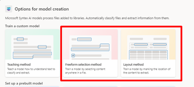
Unable to create Free form model in Syntex
Unable to create Free form model in Syntex
Hi All,
I’m trying to create these 2 models but setup got failed and showing error.
These 2 models i’m trying to create
I get this error message
I already have dataverse environment and database but still it is not allowing me to create.
Unable to create Free form model in SyntexHi All, I’m trying to create these 2 models but setup got failed and showing error. These 2 models i’m trying to create I get this error message I already have dataverse environment and database but still it is not allowing me to create. Read More
Combine 2 cells if one cell contains same text
Hi,
I want to combine the Column “Generic Name” into one cell seperated by a comma if Column “Drug Code” has the same code
As you see from the example below
Drug Code 0401000010 has 2 Generic Name
0401000010 = Amoxicillin
0401000010 = Clavulanic Acid
i want it to be combined into one cell (Coumn “Combined”)
0401000010 = Amoxicillin, Clavulanic Acid
What formula can i use to achieve this result
Thank you
DRUG CODEGeneric NameCombined0401000010AmoxicillinAmoxicillin,Clavulanic acid0401000010Clavulanic acidAmoxicillin,Clavulanic acid0401000011AmoxicillinAmoxicillin,Clavulanic acid0401000011Clavulanic acidAmoxicillin,Clavulanic acid0401000056CetirizineCetirizine, Cetirizine Hydrochloride0401000056Cetirizine HydrochlorideCetirizine, Cetirizine Hydrochloride
Hi, I want to combine the Column “Generic Name” into one cell seperated by a comma if Column “Drug Code” has the same code As you see from the example below Drug Code 0401000010 has 2 Generic Name0401000010 = Amoxicillin0401000010 = Clavulanic Acid i want it to be combined into one cell (Coumn “Combined”) 0401000010 = Amoxicillin, Clavulanic Acid What formula can i use to achieve this result Thank youDRUG CODEGeneric NameCombined0401000010AmoxicillinAmoxicillin,Clavulanic acid0401000010Clavulanic acidAmoxicillin,Clavulanic acid0401000011AmoxicillinAmoxicillin,Clavulanic acid0401000011Clavulanic acidAmoxicillin,Clavulanic acid0401000056CetirizineCetirizine, Cetirizine Hydrochloride0401000056Cetirizine HydrochlorideCetirizine, Cetirizine Hydrochloride Read More

Finetune Small Language Model (SLM) Phi-3 using Azure Machine Learning
Motivations for Small Language Models:
· Efficiency: SLMs are computationally more efficient, requiring less memory and storage, and can operate faster due to fewer parameters to process.
· Cost: Training and deploying SLMs is less expensive, making them accessible to a wider range of businesses and suitable for applications in edge computing.
· Customizability: SLMs are more adaptable to specialized applications and can be fine-tuned for specific tasks more readily than larger models· Under-Explored Potential: While large models have shown clear benefits, the potential of smaller models trained with larger datasets has been less explored. SLM aims to showcase that smaller models can achieve high performance when trained with enough data.
· Inference Efficiency: Smaller models are often more efficient during inference, which is a critical aspect when deploying models in real-world applications with resource constraints. This efficiency includes faster response times and reduces computational and energy costs.
· Accessibility for Research: By being open-source and smaller in size, SLM is more accessible to a broader range of researchers who may not have the resources to work with larger models. It provides a platform for experimentation and innovation in language model research without requiring extensive computational resources.
· Advancements in Architecture and Optimization: SLM incorporates various architectural and speed optimizations to improve computational efficiency. These enhancements allow SLM to train faster and with less memory, making it feasible to train on commonly available GPUs.
· Open-Source Contribution: The authors of SLM have made the model checkpoints and code publicly available, contributing to the open-source community and enabling further advancements and applications by others.
· End-User Applications: With its excellent performance and compact size, SLM is suitable for end-user applications, potentially even on mobile devices, providing a lightweight platform for a wide range of applications.
· Training Data and Process: SLM training process is designed to be effective and reproducible, using a mixture of natural language data and code data, aiming to make pre-training accessible and transparent.
Phi-2 (Microsoft Research)
Phi-2 is the successor of Phi-1.5, the large language model (LLM) created by Microsoft.To improve over Phi-1.5, in addition to doubling the number of parameters to 2.7 billion, Microsoft also extended the training data. Phi-2 outperforms Phi-1.5 and LLMs that are 25 times larger on several public benchmarks even though it is not aligned/fine-tuned. This is just a pre-trained model for research purposes only (non-commercial, non-revenue generating). Forget about the exorbitant fees of larger language models. Phi-2 runs efficiently on even modest hardware, democratizing access to cutting-edge AI for startups and smaller businesses. No more sky-high cloud bills, just smart, affordable solutions on your own terms. In this example, we are going to learn how to fine-tune phi-2 using QLoRA: Efficient Finetuning of Quantized LLMs with Flash Attention. QLoRA is an efficient finetuning technique that quantizes a pretrained language model to 4 bits and attaches small “Low-Rank Adapters” which are fine-tuned. This enables fine-tuning of models with up to 65 billion parameters on a single GPU; despite its efficiency, QLoRA matches the performance of full-precision fine-tuning and achieves state-of-the-art results on language tasks.
Step:1
Lets prepare the dataset. In this case we are going to download the ultrachat dataset.
from datasets import load_dataset
from random import randrange
# Load dataset from the hub
dataset = load_dataset(“HuggingFaceH4/ultrachat_200k”, split=’train_sft[:2%]’)
print(f”dataset size: {len(dataset)}”)
print(dataset[randrange(len(dataset))])
Lets take a shorter version of the dataset to create training and test example. To instruct tune our model we need to convert our structured examples into a collection of tasks described via instructions. We define a formatting_function that takes a sample and returns a string with our format instruction.
dataset = dataset.train_test_split(test_size=0.2)
train_dataset = dataset[‘train’]
train_dataset.to_json(f”data/train.jsonl”)
test_dataset = dataset[‘test’]
test_dataset.to_json(f”data/eval.jsonl”)
Lets save this training and test dataset in json format. Now let’s load the Azure ML SDK. This will help us create the necesary component.
# import required libraries
from azure.identity import DefaultAzureCredential, InteractiveBrowserCredential
from azure.ai.ml import MLClient, Input
from azure.ai.ml.dsl import pipeline
from azure.ai.ml import load_component
from azure.ai.ml import command
from azure.ai.ml.entities import Data
from azure.ai.ml import Input
from azure.ai.ml import Output
from azure.ai.ml.constants import AssetTypes
Now lets create the workspace client.
credential = DefaultAzureCredential()
workspace_ml_client = None
try:
workspace_ml_client = MLClient.from_config(credential)
except Exception as ex:
print(ex)
subscription_id= “Enter your subscription_id”
resource_group = “Enter your resource_group”
workspace= “Enter your workspace name”
workspace_ml_client = MLClient(credential, subscription_id, resource_group, workspace)
Here lets create a custom training environment.
from azure.ai.ml.entities import Environment, BuildContext
env_docker_image = Environment(
image=”mcr.microsoft.com/azureml/curated/acft-hf-nlp-gpu:latest”,
conda_file=”environment/conda.yml”,
name=”llm-training”,
description=”Environment created for llm training.”,
)
ml_client.environments.create_or_update(env_docker_image)
Let’s look at the conda.yml
name: pydata-example
channels:
– conda-forge
dependencies:
– python=3.8
– pip=21.2.4
– pip:
– bitsandbytes
– transformers
– peft
– accelerate
– einops
– datasets
Lets look at the training script. We are going to use the recently introduced method in the paper “QLoRA: Quantization-aware Low-Rank Adapter Tuning for Language Generation” by Tim Dettmers et al. QLoRA is a new technique to reduce the memory footprint of large language models during finetuning, without sacrificing performance. The TL;DR; of how QLoRA works is:
Quantize the pretrained model to 4 bits and freezing it.
Attach small, trainable adapter layers. (LoRA)
Finetune only the adapter layers, while using the frozen quantized model for context.
%%writefile src/train.py
import os
#import mlflow
import argparse
import sys
import logging
import datasets
from datasets import load_dataset
from peft import LoraConfig
import torch
import transformers
from trl import SFTTrainer
from transformers import AutoModelForCausalLM, AutoTokenizer, TrainingArguments, BitsAndBytesConfig
from datasets import load_dataset
logger = logging.getLogger(__name__)
###################
# Hyper-parameters
###################
training_config = {
“bf16”: True,
“do_eval”: False,
“learning_rate”: 5.0e-06,
“log_level”: “info”,
“logging_steps”: 20,
“logging_strategy”: “steps”,
“lr_scheduler_type”: “cosine”,
“num_train_epochs”: 1,
“max_steps”: -1,
“output_dir”: “./checkpoint_dir”,
“overwrite_output_dir”: True,
“per_device_eval_batch_size”: 4,
“per_device_train_batch_size”: 4,
“remove_unused_columns”: True,
“save_steps”: 100,
“save_total_limit”: 1,
“seed”: 0,
“gradient_checkpointing”: True,
“gradient_checkpointing_kwargs”:{“use_reentrant”: False},
“gradient_accumulation_steps”: 1,
“warmup_ratio”: 0.2,
}
peft_config = {
“r”: 16,
“lora_alpha”: 32,
“lora_dropout”: 0.05,
“bias”: “none”,
“task_type”: “CAUSAL_LM”,
“target_modules”: “all-linear”,
“modules_to_save”: None,
}
train_conf = TrainingArguments(**training_config)
peft_conf = LoraConfig(**peft_config)
###############
# Setup logging
###############
logging.basicConfig(
format=”%(asctime)s – %(levelname)s – %(name)s – %(message)s”,
datefmt=”%Y-%m-%d %H:%M:%S”,
handlers=[logging.StreamHandler(sys.stdout)],
)
log_level = train_conf.get_process_log_level()
logger.setLevel(log_level)
datasets.utils.logging.set_verbosity(log_level)
transformers.utils.logging.set_verbosity(log_level)
transformers.utils.logging.enable_default_handler()
transformers.utils.logging.enable_explicit_format()
# Log on each process a small summary
logger.warning(
f”Process rank: {train_conf.local_rank}, device: {train_conf.device}, n_gpu: {train_conf.n_gpu}”
+ f” distributed training: {bool(train_conf.local_rank != -1)}, 16-bits training: {train_conf.fp16}”
)
logger.info(f”Training/evaluation parameters {train_conf}”)
logger.info(f”PEFT parameters {peft_conf}”)
################
# Modle Loading
################
checkpoint_path = “microsoft/Phi-3-mini-4k-instruct”
# checkpoint_path = “microsoft/Phi-3-mini-128k-instruct”
model_kwargs = dict(
use_cache=False,
trust_remote_code=True,
attn_implementation=”flash_attention_2″, # loading the model with flash-attenstion support
torch_dtype=torch.bfloat16,
device_map=None
)
model = AutoModelForCausalLM.from_pretrained(checkpoint_path, **model_kwargs)
tokenizer = AutoTokenizer.from_pretrained(checkpoint_path)
tokenizer.model_max_length = 2048
tokenizer.pad_token = tokenizer.unk_token # use unk rather than eos token to prevent endless generation
tokenizer.pad_token_id = tokenizer.convert_tokens_to_ids(tokenizer.pad_token)
tokenizer.padding_side = ‘right’
##################
# Data Processing
##################
def apply_chat_template(
example,
tokenizer,
):
messages = example[“messages”]
# Add an empty system message if there is none
if messages[0][“role”] != “system”:
messages.insert(0, {“role”: “system”, “content”: “”})
example[“text”] = tokenizer.apply_chat_template(
messages, tokenize=False, add_generation_prompt=False)
return example
def main(args):
train_dataset = load_dataset(‘json’, data_files=args.train_file, split=’train’)
test_dataset = load_dataset(‘json’, data_files=args.eval_file, split=’train’)
column_names = list(train_dataset.features)
processed_train_dataset = train_dataset.map(
apply_chat_template,
fn_kwargs={“tokenizer”: tokenizer},
num_proc=10,
remove_columns=column_names,
desc=”Applying chat template to train_sft”,
)
processed_test_dataset = test_dataset.map(
apply_chat_template,
fn_kwargs={“tokenizer”: tokenizer},
num_proc=10,
remove_columns=column_names,
desc=”Applying chat template to test_sft”,
)
###########
# Training
###########
trainer = SFTTrainer(
model=model,
args=train_conf,
peft_config=peft_conf,
train_dataset=processed_train_dataset,
eval_dataset=processed_test_dataset,
max_seq_length=2048,
dataset_text_field=”text”,
tokenizer=tokenizer,
packing=True
)
train_result = trainer.train()
metrics = train_result.metrics
trainer.log_metrics(“train”, metrics)
trainer.save_metrics(“train”, metrics)
trainer.save_state()
#############
# Evaluation
#############
tokenizer.padding_side = ‘left’
metrics = trainer.evaluate()
metrics[“eval_samples”] = len(processed_test_dataset)
trainer.log_metrics(“eval”, metrics)
trainer.save_metrics(“eval”, metrics)
# ############
# # Save model
# ############
os.makedirs(args.model_dir, exist_ok=True)
torch.save(model, os.path.join(args.model_dir, “model.pt”))
def parse_args():
# setup argparse
parser = argparse.ArgumentParser()
# add arguments
parser.add_argument(“–train-file”, type=str, help=”Input data for training”)
parser.add_argument(“–eval-file”, type=str, help=”Input data for eval”)
parser.add_argument(“–model-dir”, type=str, default=”./”, help=”output directory for model”)
parser.add_argument(“–epochs”, default=10, type=int, help=”number of epochs”)
parser.add_argument(
“–batch-size”,
default=16,
type=int,
help=”mini batch size for each gpu/process”,
)
parser.add_argument(“–learning-rate”, default=0.001, type=float, help=”learning rate”)
parser.add_argument(“–momentum”, default=0.9, type=float, help=”momentum”)
parser.add_argument(
“–print-freq”,
default=200,
type=int,
help=”frequency of printing training statistics”,
)
# parse args
args = parser.parse_args()
# return args
return args
# run script
if __name__ == “__main__”:
# parse args
args = parse_args()
# call main function
main(args)
Let’s create a training compute .
from azure.ai.ml.entities import AmlCompute
# If you have a specific compute size to work with change it here. By default we use the 1 x V100 compute from the above list
compute_cluster_size = “Standard_NC6s_v3”
# If you already have a gpu cluster, mention it here. Else will create a new one with the name ‘gpu-cluster-big’
compute_cluster = “gpu-cluster”
try:
compute = ml_client.compute.get(compute_cluster)
print(“The compute cluster already exists! Reusing it for the current run”)
except Exception as ex:
print(
f”Looks like the compute cluster doesn’t exist. Creating a new one with compute size {compute_cluster_size}!”
)
try:
print(“Attempt #1 – Trying to create a dedicated compute”)
compute = AmlCompute(
name=compute_cluster,
size=compute_cluster_size,
tier=”Dedicated”,
max_instances=1, # For multi node training set this to an integer value more than 1
)
ml_client.compute.begin_create_or_update(compute).wait()
except Exception as e:
print(“Error”)
Now lets call the compute job with the above training script in the AML compute we just created.
from azure.ai.ml import command
from azure.ai.ml import Input
from azure.ai.ml.entities import ResourceConfiguration
job = command(
inputs=dict(
train_file=Input(
type=”uri_file”,
path=”data/train.jsonl”,
),
eval_file=Input(
type=”uri_file”,
path=”data/eval.jsonl”,
),
epoch=2,
batchsize=64,
lr = 0.01,
momentum = 0.9,
prtfreq = 200,
output = “./outputs”
),
code=”./src”, # local path where the code is stored
compute = ‘gpu-a100’,
command=”accelerate launch train.py –train-file ${{inputs.train_file}} –eval-file ${{inputs.eval_file}} –epochs ${{inputs.epoch}} –batch-size ${{inputs.batchsize}} –learning-rate ${{inputs.lr}} –momentum ${{inputs.momentum}} –print-freq ${{inputs.prtfreq}} –model-dir ${{inputs.output}}”,
environment=”azureml://registries/azureml/environments/acft-hf-nlp-gpu/versions/52″,
distribution={
“type”: “PyTorch”,
“process_count_per_instance”: 1,
},
)
returned_job = workspace_ml_client.jobs.create_or_update(job)
workspace_ml_client.jobs.stream(returned_job.name)
Lets look at the pipeline output.
# check if the `trained_model` output is available
job_name = returned_job.name
print(“pipeline job outputs: “, workspace_ml_client.jobs.get(job_name).outputs)
Once the model is finetuned lets register the job in the workspace to create endpoint.
from azure.ai.ml.entities import Model
from azure.ai.ml.constants import AssetTypes
run_model = Model(
path=f”azureml://jobs/{job_name}/outputs/artifacts/paths/outputs/mlflow_model_folder”,
name=”phi-3-finetuned”,
description=”Model created from run.”,
type=AssetTypes.MLFLOW_MODEL,
)
model = workspace_ml_client.models.create_or_update(run_model)
Lets creat the endpoint.
from azure.ai.ml.entities import (
ManagedOnlineEndpoint,
IdentityConfiguration,
ManagedIdentityConfiguration,
)
# Check if the endpoint already exists in the workspace
try:
endpoint = workspace_ml_client.online_endpoints.get(endpoint_name)
print(“—Endpoint already exists—“)
except:
# Create an online endpoint if it doesn’t exist
# Define the endpoint
endpoint = ManagedOnlineEndpoint(
name=endpoint_name,
description=f”Test endpoint for {model.name}”,
identity=IdentityConfiguration(
type=”user_assigned”,
user_assigned_identities=[ManagedIdentityConfiguration(resource_id=uai_id)],
)
if uai_id != “”
else None,
)
# Trigger the endpoint creation
try:
workspace_ml_client.begin_create_or_update(endpoint).wait()
print(“n—Endpoint created successfully—n”)
except Exception as err:
raise RuntimeError(
f”Endpoint creation failed. Detailed Response:n{err}”
) from err
Once the endpoint is created we can go ahead and create the deployment.
# Initialize deployment parameters
deployment_name = “phi3-deploy”
sku_name = “Standard_NCs_v3”
REQUEST_TIMEOUT_MS = 90000
deployment_env_vars = {
“SUBSCRIPTION_ID”: subscription_id,
“RESOURCE_GROUP_NAME”: resource_group,
“UAI_CLIENT_ID”: uai_client_id,
}
For inferencing we will use a different base image.
from azure.ai.ml.entities import Model, Environment
env = Environment(
image=’mcr.microsoft.com/azureml/curated/foundation-model-inference:latest’,
inference_config={
“liveness_route”: {“port”: 5001, “path”: “/”},
“readiness_route”: {“port”: 5001, “path”: “/”},
“scoring_route”: {“port”: 5001, “path”: “/score”},
},
)
Lets deploy the model
from azure.ai.ml.entities import (
OnlineRequestSettings,
CodeConfiguration,
ManagedOnlineDeployment,
ProbeSettings,
Environment
)
deployment = ManagedOnlineDeployment(
name=deployment_name,
endpoint_name=endpoint_name,
model=model.id,
instance_type=sku_name,
instance_count=1,
#code_configuration=code_configuration,
environment = env,
environment_variables=deployment_env_vars,
request_settings=OnlineRequestSettings(request_timeout_ms=REQUEST_TIMEOUT_MS),
liveness_probe=ProbeSettings(
failure_threshold=30,
success_threshold=1,
period=100,
initial_delay=500,
),
readiness_probe=ProbeSettings(
failure_threshold=30,
success_threshold=1,
period=100,
initial_delay=500,
),
)
# Trigger the deployment creation
try:
workspace_ml_client.begin_create_or_update(deployment).wait()
print(“n—Deployment created successfully—n”)
except Exception as err:
raise RuntimeError(
f”Deployment creation failed. Detailed Response:n{err}”
) from err
If you want to delete the endpoint please see the below code.
workspace_ml_client.online_deployments.begin_delete(name = deployment_name,
endpoint_name = endpoint_name)
workspace_ml_client._online_endpoints.begin_delete(name = endpoint_name)
Hope this tutorial helps you in Finetuning and deploying Phi-3 model in Azure ML Studio.
Hope you like the blog. Please clap and follow me if you like to read more such blogs coming soon.
References:
https://www.microsoft.com/en-us/research/blog/phi-2-the-surprising-power-of-small-language-models/
https://www.philschmid.de/sagemaker-falcon-180b-qlora
Microsoft Tech Community – Latest Blogs –Read More

Why should you migrate from OpenAI to Azure OpenAI?
As the field of AI continues to grow, developers are constantly seeking new and innovative ways to integrate it into their work. With the launch of Azure OpenAI Service, developers now have even more tools at their disposal to take advantage of this powerful technology. Azure OpenAI Service can be used to create chatbots, generate text, translate languages, and write different kinds of creative content. As the platform continues to evolve, developers will be able to use it to build even more powerful and sophisticated applications.
What is Azure OpenAI
Azure OpenAI Service is a fully managed service that allows developers to easily integrate OpenAI models into their applications. With Azure OpenAI Service, developers can quickly and easily access a wide range of AI models, including natural language processing, computer vision, and more. Azure OpenAI Service provides a simple and easy-to-use API that makes it easy to get started with AI
Strategic AI Provider Selection for Businesses
The AI service provider landscape is characterized by its rapid evolution and diverse offerings. Informed decision-making requires a careful analysis of the providers’ unique strengths, their pricing models, and the congruence with an organization’s specific demands and strategic ambitions.
Let’s look at some of the common scenarios in app migrations and break down major differences
Programing SDKs
Major differences we need to make to switch our apps from OpenAI to Azure OpenAI. We are going to use Python SDK for this example.
API key – The code looks similar, but Azure OpenAI adds api_version and azure_endpoint because you’re running your own instance.
Microsoft Entra ID authentication – This is helpful in adding extra security to our client instance by adding api_version, azure_endpoint and the token_provider.
Keyword argument for model – OpenAI uses the model keyword argument to specify what model to use. Azure OpenAI has the concept of unique model deployments. When you use Azure OpenAI, model should refer to the underlying deployment name you chose when you deployed the model.
Embeddings multiple input support – OpenAI and Azure OpenAI currently support input arrays up to 2,048 input items for text-embedding-ada-002. Both require the max input token limit per API request to remain under 8,191 for this model.
Other Benefits of migrating from OpenAI to Azure OpenAI
Managed Service and Infrastructure:
Azure OpenAI is a fully managed service provided by Microsoft. You don’t need to worry about setting up and maintaining infrastructure, as Azure handles it for you. You just need to spin up your OpenAI instance and start developing.
You can also configure Azure OpenAI Service with managed identities
Security and Compliance:
Azure provides robust security features, including encryption, identity management, and compliance certifications. This acts as a more friendly reason for startups, companies and organization
If your application deals with sensitive data, Azure OpenAI ensures that your models and data are protected according to industry standards. Your companied data is retained in your own Azure OpenAI instance.
Responsible AI practices for Azure OpenAI models
Azure OpenAI supported programming languages – Azure OpenAI gives you five programing languages (C#, Go, Java, JavaScript and Python) with SDKs to help you easily interact with the models.
Scalability and High Availability:
Azure’s global infrastructure allows you to scale your AI workloads dynamically. You can handle increased demand by automatically provisioning additional resources.
Azure also provides redundancy across multiple data centers, ensuring high availability and fault tolerance.
Integration with Other Azure Services:
Azure OpenAI seamlessly integrates with other Azure services, such as Azure Machine Learning, Azure Cognitive Services, and Azure Functions.
You can also build end-to-end AI pipelines by combining different services within the Azure ecosystem.
Cost Optimization:
Azure offers flexible pricing options, including pay-as-you-go (PAYG) and Provisioned Throughput Units (PTUs). With PAYG, you can optimize costs by paying only for the resources you use, while PTUs provide throughput with minimal latency variance, making them ideal for scaling your AI solutions. Each model is priced per unit, ensuring a predictable cost structure for your AI deployments.
Additionally, Azure provides cost management tools to monitor and optimize your spending. You can event approximate the cost for your Azure resources by using the Price calculator.
Read More
Migrating from OpenAI to Azure OpenAI
How to switch between OpenAI and Azure OpenAI endpoints with Python
Work with the GPT-3.5-Turbo and GPT-4 models
Azure OpenAI Service REST API reference
Quickstart: Get started generating text using Azure OpenAI Service
Azure OpenAI supported programming languages
Microsoft Tech Community – Latest Blogs –Read More

Startup Showcase: Ignitus
Making great career advice available to all
Founders Hub Benefits
Ignitus Product Demo
Connect with Ed Shee, CTO Ignitus
Join Microsoft for Startups Founders’ Hub today!
Microsoft Tech Community – Latest Blogs –Read More
color segmentation on a user-selected image using k-means clustering to identify and display different color classes, and visualizes the results with pie charts.
Hello all,
I hope you are doing well.
I need your help in adjusting this code to capture only the porosity (black shapes) that exists in the original image, instead of the inaccurate percentage results shown in the produced image and the pie chart.
I greatly appreciate your consideration.
Here is the code
% Do color segmentation by kmeans classification.
clc; % Clear the command window.
close all; % Close all figures (except those of imtool.)
clear; % Erase all existing variables. Or clearvars if you want.
workspace; % Make sure the workspace panel is showing.
format long g;
format compact;
fontSize = 16;
% Check that user has the Image Processing Toolbox installed and licensed.
hasLicenseForToolbox = license(‘test’, ‘image_toolbox’);
if ~hasLicenseForToolbox
message = sprintf(‘Sorry, but you do not seem to have the Image Processing Toolbox.nDo you want to try to continue anyway?’);
reply = questdlg(message, ‘Toolbox missing’, ‘Yes’, ‘No’, ‘Yes’);
if strcmpi(reply, ‘No’)
return;
end
end
% Check that user has the Statistics and Machine Learning Toolbox installed and licensed.
hasLicenseForToolbox = license(‘test’, ‘Statistics_toolbox’);
if ~hasLicenseForToolbox
message = sprintf(‘Sorry, but you do not seem to have the Statistics and Machine Learning Toolbox.nDo you want to try to continue anyway?’);
reply = questdlg(message, ‘Toolbox missing’, ‘Yes’, ‘No’, ‘Yes’);
if strcmpi(reply, ‘No’)
return;
end
end
% Load the specific image file
fullFileName = ‘D:\OneDrive – York University\Zeiss Microscope\Dogbone TPUDownwards\Downwards TPU Traditional Direction.jpg’;
% fullFileName = ‘D:\OneDrive – York University\Zeiss Microscope\image J\Downwards\two\Image Downwards.png’;
if ~exist(fullFileName, ‘file’)
errorMessage = sprintf(‘Error: %s does not exist.’, fullFileName);
uiwait(warndlg(errorMessage));
return;
end
rgbImage = imread(fullFileName);
% Get the dimensions of the image. numberOfColorChannels should be = 3.
[rows, columns, numberOfColorChannels] = size(rgbImage);
if numberOfColorChannels ~= 3
message = sprintf(‘You need to select an RGB image.’);
uiwait(errordlg(message));
return;
end
% Display the original color image.
subplot(2, 2, 1);
imshow(rgbImage);
title(‘Original Color Image’, ‘FontSize’, fontSize);
set(gcf, ‘Units’, ‘Normalized’, ‘Outerposition’, [0, 0, 1, 1]);
% Extract and display the color channels.
redChannel = rgbImage(:, :, 1);
greenChannel = rgbImage(:, :, 2);
blueChannel = rgbImage(:, :, 3);
subplot(2, 2, 2);
imshow(redChannel);
title(‘Red Channel’, ‘FontSize’, fontSize);
subplot(2, 2, 3);
imshow(greenChannel);
title(‘Green Channel’, ‘FontSize’, fontSize);
subplot(2, 2, 4);
imshow(blueChannel);
title(‘Blue Channel’, ‘FontSize’, fontSize);
% Ask user how many color classes they want.
defaultValue = 5;
titleBar = ‘Enter an integer value’;
userPrompt = ‘Enter the number of color classes to find (2 through 6)’;
caUserInput = inputdlg(userPrompt, titleBar, 1, {num2str(defaultValue)});
if isempty(caUserInput), return; end % Bail out if they clicked Cancel.
numberOfClasses = round(str2double(caUserInput{1}));
% Prepare data for k-means
imageData = double(reshape(rgbImage, [], 3));
indexes = kmeans(imageData, numberOfClasses);
% Reshape the cluster indexes to the original image dimensions
clusteredImage = reshape(indexes, size(rgbImage, 1), size(rgbImage, 2));
% Display clustered image
figure;
imshow(label2rgb(clusteredImage));
title(‘Clustered Image’, ‘FontSize’, fontSize);
% Calculate pixel counts for each class for the pie chart
classCounts = histcounts(indexes, 1:numberOfClasses+1);
% Create a custom color map based on the clustered image
uniqueClasses = unique(indexes);
colorsForPie = label2rgb(uniqueClasses); % Convert class numbers to RGB colors
colorsForPie = reshape(colorsForPie, [length(uniqueClasses), 3]); % Ensure it’s a Nx3 matrix for RGB
% Generate pie chart
figure;
pie(classCounts, arrayfun(@(x) sprintf(‘Class %d’, x), 1:numberOfClasses, ‘UniformOutput’, false));
colormap(colorsForPie); % Apply custom colors
% Title for pie chart
title(‘Pie Chart of Color Classes’, ‘FontSize’, fontSize);Hello all,
I hope you are doing well.
I need your help in adjusting this code to capture only the porosity (black shapes) that exists in the original image, instead of the inaccurate percentage results shown in the produced image and the pie chart.
I greatly appreciate your consideration.
Here is the code
% Do color segmentation by kmeans classification.
clc; % Clear the command window.
close all; % Close all figures (except those of imtool.)
clear; % Erase all existing variables. Or clearvars if you want.
workspace; % Make sure the workspace panel is showing.
format long g;
format compact;
fontSize = 16;
% Check that user has the Image Processing Toolbox installed and licensed.
hasLicenseForToolbox = license(‘test’, ‘image_toolbox’);
if ~hasLicenseForToolbox
message = sprintf(‘Sorry, but you do not seem to have the Image Processing Toolbox.nDo you want to try to continue anyway?’);
reply = questdlg(message, ‘Toolbox missing’, ‘Yes’, ‘No’, ‘Yes’);
if strcmpi(reply, ‘No’)
return;
end
end
% Check that user has the Statistics and Machine Learning Toolbox installed and licensed.
hasLicenseForToolbox = license(‘test’, ‘Statistics_toolbox’);
if ~hasLicenseForToolbox
message = sprintf(‘Sorry, but you do not seem to have the Statistics and Machine Learning Toolbox.nDo you want to try to continue anyway?’);
reply = questdlg(message, ‘Toolbox missing’, ‘Yes’, ‘No’, ‘Yes’);
if strcmpi(reply, ‘No’)
return;
end
end
% Load the specific image file
fullFileName = ‘D:\OneDrive – York University\Zeiss Microscope\Dogbone TPUDownwards\Downwards TPU Traditional Direction.jpg’;
% fullFileName = ‘D:\OneDrive – York University\Zeiss Microscope\image J\Downwards\two\Image Downwards.png’;
if ~exist(fullFileName, ‘file’)
errorMessage = sprintf(‘Error: %s does not exist.’, fullFileName);
uiwait(warndlg(errorMessage));
return;
end
rgbImage = imread(fullFileName);
% Get the dimensions of the image. numberOfColorChannels should be = 3.
[rows, columns, numberOfColorChannels] = size(rgbImage);
if numberOfColorChannels ~= 3
message = sprintf(‘You need to select an RGB image.’);
uiwait(errordlg(message));
return;
end
% Display the original color image.
subplot(2, 2, 1);
imshow(rgbImage);
title(‘Original Color Image’, ‘FontSize’, fontSize);
set(gcf, ‘Units’, ‘Normalized’, ‘Outerposition’, [0, 0, 1, 1]);
% Extract and display the color channels.
redChannel = rgbImage(:, :, 1);
greenChannel = rgbImage(:, :, 2);
blueChannel = rgbImage(:, :, 3);
subplot(2, 2, 2);
imshow(redChannel);
title(‘Red Channel’, ‘FontSize’, fontSize);
subplot(2, 2, 3);
imshow(greenChannel);
title(‘Green Channel’, ‘FontSize’, fontSize);
subplot(2, 2, 4);
imshow(blueChannel);
title(‘Blue Channel’, ‘FontSize’, fontSize);
% Ask user how many color classes they want.
defaultValue = 5;
titleBar = ‘Enter an integer value’;
userPrompt = ‘Enter the number of color classes to find (2 through 6)’;
caUserInput = inputdlg(userPrompt, titleBar, 1, {num2str(defaultValue)});
if isempty(caUserInput), return; end % Bail out if they clicked Cancel.
numberOfClasses = round(str2double(caUserInput{1}));
% Prepare data for k-means
imageData = double(reshape(rgbImage, [], 3));
indexes = kmeans(imageData, numberOfClasses);
% Reshape the cluster indexes to the original image dimensions
clusteredImage = reshape(indexes, size(rgbImage, 1), size(rgbImage, 2));
% Display clustered image
figure;
imshow(label2rgb(clusteredImage));
title(‘Clustered Image’, ‘FontSize’, fontSize);
% Calculate pixel counts for each class for the pie chart
classCounts = histcounts(indexes, 1:numberOfClasses+1);
% Create a custom color map based on the clustered image
uniqueClasses = unique(indexes);
colorsForPie = label2rgb(uniqueClasses); % Convert class numbers to RGB colors
colorsForPie = reshape(colorsForPie, [length(uniqueClasses), 3]); % Ensure it’s a Nx3 matrix for RGB
% Generate pie chart
figure;
pie(classCounts, arrayfun(@(x) sprintf(‘Class %d’, x), 1:numberOfClasses, ‘UniformOutput’, false));
colormap(colorsForPie); % Apply custom colors
% Title for pie chart
title(‘Pie Chart of Color Classes’, ‘FontSize’, fontSize); Hello all,
I hope you are doing well.
I need your help in adjusting this code to capture only the porosity (black shapes) that exists in the original image, instead of the inaccurate percentage results shown in the produced image and the pie chart.
I greatly appreciate your consideration.
Here is the code
% Do color segmentation by kmeans classification.
clc; % Clear the command window.
close all; % Close all figures (except those of imtool.)
clear; % Erase all existing variables. Or clearvars if you want.
workspace; % Make sure the workspace panel is showing.
format long g;
format compact;
fontSize = 16;
% Check that user has the Image Processing Toolbox installed and licensed.
hasLicenseForToolbox = license(‘test’, ‘image_toolbox’);
if ~hasLicenseForToolbox
message = sprintf(‘Sorry, but you do not seem to have the Image Processing Toolbox.nDo you want to try to continue anyway?’);
reply = questdlg(message, ‘Toolbox missing’, ‘Yes’, ‘No’, ‘Yes’);
if strcmpi(reply, ‘No’)
return;
end
end
% Check that user has the Statistics and Machine Learning Toolbox installed and licensed.
hasLicenseForToolbox = license(‘test’, ‘Statistics_toolbox’);
if ~hasLicenseForToolbox
message = sprintf(‘Sorry, but you do not seem to have the Statistics and Machine Learning Toolbox.nDo you want to try to continue anyway?’);
reply = questdlg(message, ‘Toolbox missing’, ‘Yes’, ‘No’, ‘Yes’);
if strcmpi(reply, ‘No’)
return;
end
end
% Load the specific image file
fullFileName = ‘D:\OneDrive – York University\Zeiss Microscope\Dogbone TPUDownwards\Downwards TPU Traditional Direction.jpg’;
% fullFileName = ‘D:\OneDrive – York University\Zeiss Microscope\image J\Downwards\two\Image Downwards.png’;
if ~exist(fullFileName, ‘file’)
errorMessage = sprintf(‘Error: %s does not exist.’, fullFileName);
uiwait(warndlg(errorMessage));
return;
end
rgbImage = imread(fullFileName);
% Get the dimensions of the image. numberOfColorChannels should be = 3.
[rows, columns, numberOfColorChannels] = size(rgbImage);
if numberOfColorChannels ~= 3
message = sprintf(‘You need to select an RGB image.’);
uiwait(errordlg(message));
return;
end
% Display the original color image.
subplot(2, 2, 1);
imshow(rgbImage);
title(‘Original Color Image’, ‘FontSize’, fontSize);
set(gcf, ‘Units’, ‘Normalized’, ‘Outerposition’, [0, 0, 1, 1]);
% Extract and display the color channels.
redChannel = rgbImage(:, :, 1);
greenChannel = rgbImage(:, :, 2);
blueChannel = rgbImage(:, :, 3);
subplot(2, 2, 2);
imshow(redChannel);
title(‘Red Channel’, ‘FontSize’, fontSize);
subplot(2, 2, 3);
imshow(greenChannel);
title(‘Green Channel’, ‘FontSize’, fontSize);
subplot(2, 2, 4);
imshow(blueChannel);
title(‘Blue Channel’, ‘FontSize’, fontSize);
% Ask user how many color classes they want.
defaultValue = 5;
titleBar = ‘Enter an integer value’;
userPrompt = ‘Enter the number of color classes to find (2 through 6)’;
caUserInput = inputdlg(userPrompt, titleBar, 1, {num2str(defaultValue)});
if isempty(caUserInput), return; end % Bail out if they clicked Cancel.
numberOfClasses = round(str2double(caUserInput{1}));
% Prepare data for k-means
imageData = double(reshape(rgbImage, [], 3));
indexes = kmeans(imageData, numberOfClasses);
% Reshape the cluster indexes to the original image dimensions
clusteredImage = reshape(indexes, size(rgbImage, 1), size(rgbImage, 2));
% Display clustered image
figure;
imshow(label2rgb(clusteredImage));
title(‘Clustered Image’, ‘FontSize’, fontSize);
% Calculate pixel counts for each class for the pie chart
classCounts = histcounts(indexes, 1:numberOfClasses+1);
% Create a custom color map based on the clustered image
uniqueClasses = unique(indexes);
colorsForPie = label2rgb(uniqueClasses); % Convert class numbers to RGB colors
colorsForPie = reshape(colorsForPie, [length(uniqueClasses), 3]); % Ensure it’s a Nx3 matrix for RGB
% Generate pie chart
figure;
pie(classCounts, arrayfun(@(x) sprintf(‘Class %d’, x), 1:numberOfClasses, ‘UniformOutput’, false));
colormap(colorsForPie); % Apply custom colors
% Title for pie chart
title(‘Pie Chart of Color Classes’, ‘FontSize’, fontSize); dbscan, kmeans, clustering MATLAB Answers — New Questions
Create a matrix and a map of Hydrologic Soil Group values using integer or character values
I want to create a matrix and a map of Hydrologic Soil Group (HSG) values using integer or character values. I have a vector of 8853×1 with the HSG letters (A, B, C or D) for different locations in St. Croix island (USVI). I want to produce a 102×263 matrix with those letters, using different scripts that I have available. The problem is that Matlab doesn’t let me produce a matrix with letters or character values (char format). The thing is, if I use numbers instead of letters (1, 2, 3 and 4), the matrix that is produced has all the numbers in double or float format, with decimal digits, and not whole numbers or integers.. But when I converted the vector to integer format, matlab doesn’t produce a matrix from that vector. I will use this matrix to plot a map of the island showing different colors according to the HSG values or letters. How can I produce a matrix and a map with integer and/or character values using a 8853×1 vector? Should I just round up the numbers in the matrix to the nearest whole number?I want to create a matrix and a map of Hydrologic Soil Group (HSG) values using integer or character values. I have a vector of 8853×1 with the HSG letters (A, B, C or D) for different locations in St. Croix island (USVI). I want to produce a 102×263 matrix with those letters, using different scripts that I have available. The problem is that Matlab doesn’t let me produce a matrix with letters or character values (char format). The thing is, if I use numbers instead of letters (1, 2, 3 and 4), the matrix that is produced has all the numbers in double or float format, with decimal digits, and not whole numbers or integers.. But when I converted the vector to integer format, matlab doesn’t produce a matrix from that vector. I will use this matrix to plot a map of the island showing different colors according to the HSG values or letters. How can I produce a matrix and a map with integer and/or character values using a 8853×1 vector? Should I just round up the numbers in the matrix to the nearest whole number? I want to create a matrix and a map of Hydrologic Soil Group (HSG) values using integer or character values. I have a vector of 8853×1 with the HSG letters (A, B, C or D) for different locations in St. Croix island (USVI). I want to produce a 102×263 matrix with those letters, using different scripts that I have available. The problem is that Matlab doesn’t let me produce a matrix with letters or character values (char format). The thing is, if I use numbers instead of letters (1, 2, 3 and 4), the matrix that is produced has all the numbers in double or float format, with decimal digits, and not whole numbers or integers.. But when I converted the vector to integer format, matlab doesn’t produce a matrix from that vector. I will use this matrix to plot a map of the island showing different colors according to the HSG values or letters. How can I produce a matrix and a map with integer and/or character values using a 8853×1 vector? Should I just round up the numbers in the matrix to the nearest whole number? matrix array, colormap, vectors MATLAB Answers — New Questions
Why is my variable being changed without assignment
Hello,
I have searched quite a lot on Google and cannot find anything related to what is happening, and just in general programming terms I cannot understand it either. I’m stumped and hope someone can shed some light. An analogy of what seems to be happening is this:
A = 1
B = A + 2 = 3 (and now A = 3!!!)
This makes no sense to me, how can the original value of A be getting changed without. This is my first time using Live Script and symbols, so perhaps there is something different around those concepts.
My code is below. The issue is that when I substitute 0 into yh(zero), it is also changing the value of yh. Thus when I perform a subs to calc yhNat (last line), the value it is referencing is no longer yh but actually yh(zero). If I leave out the calc of yh(zero) then yhNat calculates perfectly (15*exp((-2*t)) + 16*exp((-3*t))). The only thing I can think of is because the initial value assigned to both yh and yh(zero) is the same, perhaps Matlab is conflating/linking them somehow. Originally I just made yh(zero) a subs of yh, replacing all t’s with 0, but that didn’t work, hence the workaround.
Any help would be greatly appreciated, as I am fully stuck and all my years of messing around with programming languages aren’t helping at all to understand why this is happening.
% Homogenous solution
InitialVoltage = 1.5;
InitialCurrent = 2;
c_UD = 1/6;
%from earlier code roots.1 = -3, roots.2 = -2
syms yh yh(zero) yhNat dyh(t) dyh(zero) c_1 c_2
yh = c_1*exp(roots(1)*t) + c_2*exp(roots(2)*t)
dyh(t) = diff(yh)
dyh(zero) = subs(dyh(t),[t],[0]) == InitialCurrent/c_UD
%Evaluate yh(t) at t = 0:
yh(zero) = c_1*exp(roots(1)*t) + c_2*exp(roots(2)*t); %######### These two lines break it
yh(zero) = subs(yh(zero), [t], [0]) == vpa(InitialVoltage) %######### These two lines break it
%coefficients = solve([dyh(zero), yh(zero)], [c_1, c_2])
%Natural response
yhNat = subs(yh ,[c_1, c_2], [16, 15])Hello,
I have searched quite a lot on Google and cannot find anything related to what is happening, and just in general programming terms I cannot understand it either. I’m stumped and hope someone can shed some light. An analogy of what seems to be happening is this:
A = 1
B = A + 2 = 3 (and now A = 3!!!)
This makes no sense to me, how can the original value of A be getting changed without. This is my first time using Live Script and symbols, so perhaps there is something different around those concepts.
My code is below. The issue is that when I substitute 0 into yh(zero), it is also changing the value of yh. Thus when I perform a subs to calc yhNat (last line), the value it is referencing is no longer yh but actually yh(zero). If I leave out the calc of yh(zero) then yhNat calculates perfectly (15*exp((-2*t)) + 16*exp((-3*t))). The only thing I can think of is because the initial value assigned to both yh and yh(zero) is the same, perhaps Matlab is conflating/linking them somehow. Originally I just made yh(zero) a subs of yh, replacing all t’s with 0, but that didn’t work, hence the workaround.
Any help would be greatly appreciated, as I am fully stuck and all my years of messing around with programming languages aren’t helping at all to understand why this is happening.
% Homogenous solution
InitialVoltage = 1.5;
InitialCurrent = 2;
c_UD = 1/6;
%from earlier code roots.1 = -3, roots.2 = -2
syms yh yh(zero) yhNat dyh(t) dyh(zero) c_1 c_2
yh = c_1*exp(roots(1)*t) + c_2*exp(roots(2)*t)
dyh(t) = diff(yh)
dyh(zero) = subs(dyh(t),[t],[0]) == InitialCurrent/c_UD
%Evaluate yh(t) at t = 0:
yh(zero) = c_1*exp(roots(1)*t) + c_2*exp(roots(2)*t); %######### These two lines break it
yh(zero) = subs(yh(zero), [t], [0]) == vpa(InitialVoltage) %######### These two lines break it
%coefficients = solve([dyh(zero), yh(zero)], [c_1, c_2])
%Natural response
yhNat = subs(yh ,[c_1, c_2], [16, 15]) Hello,
I have searched quite a lot on Google and cannot find anything related to what is happening, and just in general programming terms I cannot understand it either. I’m stumped and hope someone can shed some light. An analogy of what seems to be happening is this:
A = 1
B = A + 2 = 3 (and now A = 3!!!)
This makes no sense to me, how can the original value of A be getting changed without. This is my first time using Live Script and symbols, so perhaps there is something different around those concepts.
My code is below. The issue is that when I substitute 0 into yh(zero), it is also changing the value of yh. Thus when I perform a subs to calc yhNat (last line), the value it is referencing is no longer yh but actually yh(zero). If I leave out the calc of yh(zero) then yhNat calculates perfectly (15*exp((-2*t)) + 16*exp((-3*t))). The only thing I can think of is because the initial value assigned to both yh and yh(zero) is the same, perhaps Matlab is conflating/linking them somehow. Originally I just made yh(zero) a subs of yh, replacing all t’s with 0, but that didn’t work, hence the workaround.
Any help would be greatly appreciated, as I am fully stuck and all my years of messing around with programming languages aren’t helping at all to understand why this is happening.
% Homogenous solution
InitialVoltage = 1.5;
InitialCurrent = 2;
c_UD = 1/6;
%from earlier code roots.1 = -3, roots.2 = -2
syms yh yh(zero) yhNat dyh(t) dyh(zero) c_1 c_2
yh = c_1*exp(roots(1)*t) + c_2*exp(roots(2)*t)
dyh(t) = diff(yh)
dyh(zero) = subs(dyh(t),[t],[0]) == InitialCurrent/c_UD
%Evaluate yh(t) at t = 0:
yh(zero) = c_1*exp(roots(1)*t) + c_2*exp(roots(2)*t); %######### These two lines break it
yh(zero) = subs(yh(zero), [t], [0]) == vpa(InitialVoltage) %######### These two lines break it
%coefficients = solve([dyh(zero), yh(zero)], [c_1, c_2])
%Natural response
yhNat = subs(yh ,[c_1, c_2], [16, 15]) live script, variable assignment MATLAB Answers — New Questions
How do I use All Video Downloader for PC Windows 10?
I’m trying to get a handle on using an All Video Downloader on my PC, but I’m not quite sure where to start. I’ve downloaded a few apps that claim to do the job, but I’m struggling with the setup and how to actually use them effectively. Can anyone share their experiences or provide a step-by-step guide on how to use these types of programs? Specifically, I’m looking to download videos from various platforms and would appreciate any advice on making the process smooth and efficient.
I’m trying to get a handle on using an All Video Downloader on my PC, but I’m not quite sure where to start. I’ve downloaded a few apps that claim to do the job, but I’m struggling with the setup and how to actually use them effectively. Can anyone share their experiences or provide a step-by-step guide on how to use these types of programs? Specifically, I’m looking to download videos from various platforms and would appreciate any advice on making the process smooth and efficient. Read More
I have difficulty using bird’s eye scope..
I am trying to add seonsors and simulate my roadrunner scenario using matlab.
I copied the commands in mathworks, but it doesn’t work. There’s an error at line 30 (about Bird’s eye scope)..
How can I sove this? please help me…I am trying to add seonsors and simulate my roadrunner scenario using matlab.
I copied the commands in mathworks, but it doesn’t work. There’s an error at line 30 (about Bird’s eye scope)..
How can I sove this? please help me… I am trying to add seonsors and simulate my roadrunner scenario using matlab.
I copied the commands in mathworks, but it doesn’t work. There’s an error at line 30 (about Bird’s eye scope)..
How can I sove this? please help me… roadrunner, bep, bird’s eye scope, matlab, error, seonsor, scenario, simulate MATLAB Answers — New Questions
Why is the scope of output of Liquid level system here showing a straight line and not an exponential like a step?
My components have been modelled as per image1.png
However, the output that I am getting when I click on scope and run looks like a straight line and not an exponential.
According to the book from which I am learning, it was supposed to be an exponential.
I have attached the slx file as well. Can someone explain why I am not getting an exponential as output?My components have been modelled as per image1.png
However, the output that I am getting when I click on scope and run looks like a straight line and not an exponential.
According to the book from which I am learning, it was supposed to be an exponential.
I have attached the slx file as well. Can someone explain why I am not getting an exponential as output? My components have been modelled as per image1.png
However, the output that I am getting when I click on scope and run looks like a straight line and not an exponential.
According to the book from which I am learning, it was supposed to be an exponential.
I have attached the slx file as well. Can someone explain why I am not getting an exponential as output? simulink, graph, model, control, transfer function MATLAB Answers — New Questions
(Strain vs Stress Curve) to (Stress Vs Strain Curve) Switch My X-axis into Y-axis in my plot
I plotted a strain- stress curve graph however, in physical materials studies stress(y-axis)-strain(x-axis) curve is the convention in plotting. I have tried to change the graph axis but to just recive a blank plot. I have tried everything but to no avail. What am I doing wrong?
clc
clear all
close all
E1=4000; %4GPa written in 4000 MPa
E2=5000; %5GPa written in 5000 MPa
Mu= 1.2*10^5; %this measures creep
stress0.norm = 800; %this is initial stress value is in MPa
for i=1:stress0.norm
strain.normal(i)=i/E1; % This is storing the values before yielding
end
for i=stress0.norm:1500 %this is the finising stress in MPa (after yielding
strain.normal(i)=(i/E1)+((i-stress0.norm)/E2); % This is storing the values after yielding
end
% The graph with what I started off
figure (‘Name’, ‘Linear Hardening Model’, ‘NumberTitle’, ‘off’)
plot (strain.normal,’b’);
hold on
plot (800,.2, ‘rx’, ‘LineWidth’, 2);
% plot (strain.normal,’b’);
title (‘Linear Hardening Model E2 +/- 10%’);
xticks(0:100:1500);
xlabel(‘stress(in MPa)’);
ylabel(‘strain’);
grid on
legend(‘Normal’,’Yielding Location’,’Location’,’NorthEast’)
% What I wanted to achieve but get a blank graph
figure (‘Name’, ‘Linear Hardening Models Issue ‘, ‘NumberTitle’, ‘off’)
plot (strain.normal,length(strain.normal),’b’);
hold on
plot (.2,800,’rx’, ‘LineWidth’, 2);
title (‘Linear Hardening Model’);
axis ([0 0.6 0 1500])
yticks(0:100:1500);
xticks
xlabel(‘strain’);
ylabel(‘stress(in MPa)’);
grid on
legend(‘Normal’,’Yielding Location’,’Location’,’NorthEast’)I plotted a strain- stress curve graph however, in physical materials studies stress(y-axis)-strain(x-axis) curve is the convention in plotting. I have tried to change the graph axis but to just recive a blank plot. I have tried everything but to no avail. What am I doing wrong?
clc
clear all
close all
E1=4000; %4GPa written in 4000 MPa
E2=5000; %5GPa written in 5000 MPa
Mu= 1.2*10^5; %this measures creep
stress0.norm = 800; %this is initial stress value is in MPa
for i=1:stress0.norm
strain.normal(i)=i/E1; % This is storing the values before yielding
end
for i=stress0.norm:1500 %this is the finising stress in MPa (after yielding
strain.normal(i)=(i/E1)+((i-stress0.norm)/E2); % This is storing the values after yielding
end
% The graph with what I started off
figure (‘Name’, ‘Linear Hardening Model’, ‘NumberTitle’, ‘off’)
plot (strain.normal,’b’);
hold on
plot (800,.2, ‘rx’, ‘LineWidth’, 2);
% plot (strain.normal,’b’);
title (‘Linear Hardening Model E2 +/- 10%’);
xticks(0:100:1500);
xlabel(‘stress(in MPa)’);
ylabel(‘strain’);
grid on
legend(‘Normal’,’Yielding Location’,’Location’,’NorthEast’)
% What I wanted to achieve but get a blank graph
figure (‘Name’, ‘Linear Hardening Models Issue ‘, ‘NumberTitle’, ‘off’)
plot (strain.normal,length(strain.normal),’b’);
hold on
plot (.2,800,’rx’, ‘LineWidth’, 2);
title (‘Linear Hardening Model’);
axis ([0 0.6 0 1500])
yticks(0:100:1500);
xticks
xlabel(‘strain’);
ylabel(‘stress(in MPa)’);
grid on
legend(‘Normal’,’Yielding Location’,’Location’,’NorthEast’) I plotted a strain- stress curve graph however, in physical materials studies stress(y-axis)-strain(x-axis) curve is the convention in plotting. I have tried to change the graph axis but to just recive a blank plot. I have tried everything but to no avail. What am I doing wrong?
clc
clear all
close all
E1=4000; %4GPa written in 4000 MPa
E2=5000; %5GPa written in 5000 MPa
Mu= 1.2*10^5; %this measures creep
stress0.norm = 800; %this is initial stress value is in MPa
for i=1:stress0.norm
strain.normal(i)=i/E1; % This is storing the values before yielding
end
for i=stress0.norm:1500 %this is the finising stress in MPa (after yielding
strain.normal(i)=(i/E1)+((i-stress0.norm)/E2); % This is storing the values after yielding
end
% The graph with what I started off
figure (‘Name’, ‘Linear Hardening Model’, ‘NumberTitle’, ‘off’)
plot (strain.normal,’b’);
hold on
plot (800,.2, ‘rx’, ‘LineWidth’, 2);
% plot (strain.normal,’b’);
title (‘Linear Hardening Model E2 +/- 10%’);
xticks(0:100:1500);
xlabel(‘stress(in MPa)’);
ylabel(‘strain’);
grid on
legend(‘Normal’,’Yielding Location’,’Location’,’NorthEast’)
% What I wanted to achieve but get a blank graph
figure (‘Name’, ‘Linear Hardening Models Issue ‘, ‘NumberTitle’, ‘off’)
plot (strain.normal,length(strain.normal),’b’);
hold on
plot (.2,800,’rx’, ‘LineWidth’, 2);
title (‘Linear Hardening Model’);
axis ([0 0.6 0 1500])
yticks(0:100:1500);
xticks
xlabel(‘strain’);
ylabel(‘stress(in MPa)’);
grid on
legend(‘Normal’,’Yielding Location’,’Location’,’NorthEast’) mechanics, materials science, plotting, axis MATLAB Answers — New Questions
Access FPGA External Memory Using AXI Manager over PCI Express Implement
I tried to follow the example:
Access FPGA External Memory Using AXI Manager over PCI Express – MATLAB & Simulink Example (mathworks.com)
I finished generating the bitstream file, programmed it to the board and then restarted.
When I used h = aximanager(‘Xilinx’,’ interface’,’pcie’); command, the following error occurs:
Error using pciexilinx_mex
Error: There is no compatibility FPGA-in-the-Loop device in the system. You may have not installed the driver required for this operation.
Error in hdlverifier.AXIManagerPCIe/openPCIeConnection
Error in hdlverifier.AXIManagerPCIe
Error in aximanager
Later I thought that I did not install the XDMA driver. After I installed it, the problem was still the same. I would like to ask how to solve this?
I implemented it with vivado 2022.2, matlab R2023b, KCU116 fpga board on windows.I tried to follow the example:
Access FPGA External Memory Using AXI Manager over PCI Express – MATLAB & Simulink Example (mathworks.com)
I finished generating the bitstream file, programmed it to the board and then restarted.
When I used h = aximanager(‘Xilinx’,’ interface’,’pcie’); command, the following error occurs:
Error using pciexilinx_mex
Error: There is no compatibility FPGA-in-the-Loop device in the system. You may have not installed the driver required for this operation.
Error in hdlverifier.AXIManagerPCIe/openPCIeConnection
Error in hdlverifier.AXIManagerPCIe
Error in aximanager
Later I thought that I did not install the XDMA driver. After I installed it, the problem was still the same. I would like to ask how to solve this?
I implemented it with vivado 2022.2, matlab R2023b, KCU116 fpga board on windows. I tried to follow the example:
Access FPGA External Memory Using AXI Manager over PCI Express – MATLAB & Simulink Example (mathworks.com)
I finished generating the bitstream file, programmed it to the board and then restarted.
When I used h = aximanager(‘Xilinx’,’ interface’,’pcie’); command, the following error occurs:
Error using pciexilinx_mex
Error: There is no compatibility FPGA-in-the-Loop device in the system. You may have not installed the driver required for this operation.
Error in hdlverifier.AXIManagerPCIe/openPCIeConnection
Error in hdlverifier.AXIManagerPCIe
Error in aximanager
Later I thought that I did not install the XDMA driver. After I installed it, the problem was still the same. I would like to ask how to solve this?
I implemented it with vivado 2022.2, matlab R2023b, KCU116 fpga board on windows. axi manager over pci express, fil, pciexilinx_mex MATLAB Answers — New Questions
How to assign a value to a variable in an equation
Hi
I have an equation and I want to assign a value to its variable
I wrote the code below but it didn’t change after running the code what can I do
Thanks
My code
clc
clear all
close all
warning off
zafar_queue =readtable(‘zafar_queue.xlsx’);
Y = zafar_queue.nVehContrib;
data = Y’;
x_train = floor(0.9*numel(data));
dataTrain =data(1:x_train);
n = length(dataTrain);
u = 0.1* randn(n,1) ;
% Import mydata
Opt = arxOptions;
Opt.InitialCondition = ‘estimate’;
arx30 = @(z)ar(dataTrain,[30], Opt)
z = Y(end)
frcast = arx30(z)
The result after compiling code is above without caculating z in itHi
I have an equation and I want to assign a value to its variable
I wrote the code below but it didn’t change after running the code what can I do
Thanks
My code
clc
clear all
close all
warning off
zafar_queue =readtable(‘zafar_queue.xlsx’);
Y = zafar_queue.nVehContrib;
data = Y’;
x_train = floor(0.9*numel(data));
dataTrain =data(1:x_train);
n = length(dataTrain);
u = 0.1* randn(n,1) ;
% Import mydata
Opt = arxOptions;
Opt.InitialCondition = ‘estimate’;
arx30 = @(z)ar(dataTrain,[30], Opt)
z = Y(end)
frcast = arx30(z)
The result after compiling code is above without caculating z in it Hi
I have an equation and I want to assign a value to its variable
I wrote the code below but it didn’t change after running the code what can I do
Thanks
My code
clc
clear all
close all
warning off
zafar_queue =readtable(‘zafar_queue.xlsx’);
Y = zafar_queue.nVehContrib;
data = Y’;
x_train = floor(0.9*numel(data));
dataTrain =data(1:x_train);
n = length(dataTrain);
u = 0.1* randn(n,1) ;
% Import mydata
Opt = arxOptions;
Opt.InitialCondition = ‘estimate’;
arx30 = @(z)ar(dataTrain,[30], Opt)
z = Y(end)
frcast = arx30(z)
The result after compiling code is above without caculating z in it variable, equation, assign MATLAB Answers — New Questions
Duration decreases when asign more than one work resource
I have a problem with project, when asign more than one work resource to a fixed units task, the duration is decreased by project. It did not happen before.
It reduce duration! it shouldnt do that the duration should have been the same.
How can I fix this problem????
Thanks in advance for your help
I have a problem with project, when asign more than one work resource to a fixed units task, the duration is decreased by project. It did not happen before.It reduce duration! it shouldnt do that the duration should have been the same.How can I fix this problem????Thanks in advance for your help Read More
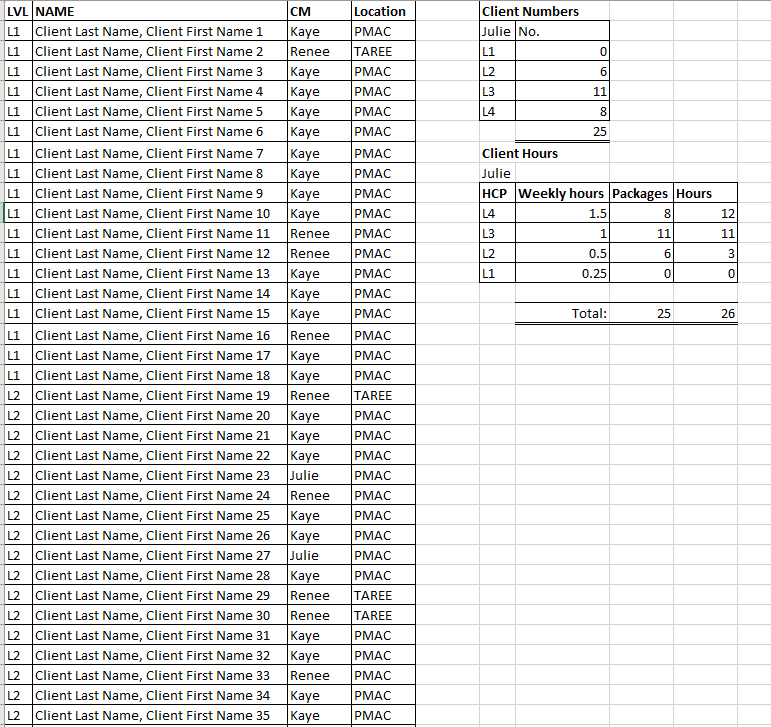
Looking for help! – lookup
Hi Excel Community!
I’m looking for some help for an Excel beginner. I have a spreadsheet for client management hours for my team, and currently, we’re calculating everything manually.
I’ve done some googling and found some suggested formulas for lookup tools, etc., but I’m not sure if this is the right path.
Basically, we have a list of clients that we sort into levels per manager, which is calculated, and then we calculate hours per week based on those levels.
I’d ideally like each manager to enter their client onto this sheet and have it automatically add to both totals (client numbers and client hours)
I’ve attached an example to explain my use/needs better.
Hoping someone can assist me or give me some ideas 🙂
Hi Excel Community! I’m looking for some help for an Excel beginner. I have a spreadsheet for client management hours for my team, and currently, we’re calculating everything manually. I’ve done some googling and found some suggested formulas for lookup tools, etc., but I’m not sure if this is the right path. Basically, we have a list of clients that we sort into levels per manager, which is calculated, and then we calculate hours per week based on those levels. I’d ideally like each manager to enter their client onto this sheet and have it automatically add to both totals (client numbers and client hours) I’ve attached an example to explain my use/needs better. Hoping someone can assist me or give me some ideas 🙂 Read More
How do I download Instagram video to mp4 on Windows 11?
Hi folks! I’m stuck trying to download videos from Instagram and save Instagram video to MP4s on my Windows 11 laptop. I’ve hit a few dead ends with methods I found online, and nothing seems to stick. Is there a secret sauce or a go-to tool I’m not aware of? Would really appreciate it if someone could point me in the right direction. Cheers for any help you can give!
Hi folks! I’m stuck trying to download videos from Instagram and save Instagram video to MP4s on my Windows 11 laptop. I’ve hit a few dead ends with methods I found online, and nothing seems to stick. Is there a secret sauce or a go-to tool I’m not aware of? Would really appreciate it if someone could point me in the right direction. Cheers for any help you can give! Read More
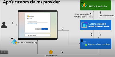
Basic understanding on Microsoft Entra custom claims provider
TOC
What is it
Architecture
How to use it
References
What is it
When a user authenticates to an app (e.g., MS Entra ID application), a custom claims provider can be used to add claims into the token. A custom claims provider is made up of a custom authentication extension that calls an external REST API (e.g., a Function App), to fetch claims from external systems (e.g., a Database). A custom claims provider can be assigned to one or many applications.
Claim: Please imagine it as features (or attributes) that belong to the end user. As it may involve sensitive information within the enterprise, the enterprise owner wishes to store this user information in the on-premises environment, while also hoping to retrieve and utilize it through the authentication process.
This service is suitable for the following scenarios:
1) It can be used as a transition for gradually migrating on-premises Active Directory to Microsoft Azure AD.
2) When user-sensitive information needs to be stored in an on-premises environment for various reasons.
Architecture
Procedure:
User login to the Application
If this AAD includes a custom claims provider, then the relevant features need to be obtained from the custom claims provider before generating the token.
The Custom claims provider asking our own system (e.g., a Function App) for the claims (e.g., criminal record) related to that user.
Our system get the related claims (e.g., by querying DB) and return it to the Custom claims provider.
The custom claims provider packages the default user information along with the additionally obtained claims, encodes them into a token, and returns it to the user.
How to use it
A-1: Create a Function App from Azure portal
Choose “.NET 6 (LTS), in-process model” as the runtime and “Windows” as the OS.
A-2: Setup a local project via VSCode
Open VSCode.
Create a new folder for your project (e.g., ccp-func)
Under the Workspace bar, select the Azure Functions icon > Create New Project.
Select C# as the language, and .NET 6.0 LTS as the .NET runtime.
Select HTTP trigger as the template.
Provide a name for the trigger (e.g., AuthEventsTrigger)
Accept Company.Function as the namespace, with AccessRights set to Function.
Open the terminal, navigate to the project folder and enter the following:
dotnet add package Microsoft.Azure.WebJobs.Extensions.AuthenticationEvents –prerelease
A-3: Add/Modify the sample code
Open the *.csproj file, change the AuthenticationEvents version to “1.0.0-beta.6”
Open the AuthEventsTrigger.cs file, copy and paste the following code to replace
using System;
using System.Threading.Tasks;
using Microsoft.AspNetCore.Mvc;
using Microsoft.Azure.WebJobs;
using Microsoft.Extensions.Logging;
using Microsoft.Azure.WebJobs.Extensions.AuthenticationEvents.TokenIssuanceStart.Actions;
using Microsoft.Azure.WebJobs.Extensions.AuthenticationEvents.TokenIssuanceStart;
using Microsoft.Azure.WebJobs.Extensions.AuthenticationEvents.Framework;
using Microsoft.Azure.WebJobs.Extensions.AuthenticationEvents;
namespace AuthEventTrigger
{
public static class Function1
{
[FunctionName(“onTokenIssuanceStart”)]
public static AuthenticationEventResponse Run(
[AuthenticationEventsTrigger(AudienceAppId = “TBA”,
AuthorityUrl = “https://login.microsoftonline.com/TBA”,
AuthorizedPartyAppId = “99045fe1-7639-4a75-9d4a-577b6ca3810f”)]TokenIssuanceStartRequest request, ILogger log)
{
try
{
if (request.RequestStatus == RequestStatusType.Successful)
{
request.Response.Actions.Add(new ProvideClaimsForToken(
new TokenClaim(“dateOfBirth”, “01/01/2000”),
new TokenClaim(“customRoles”, “Writer”, “Editor”),
new TokenClaim(“apiVersion”, “1.0.0”),
new TokenClaim(“correlationId”, request.Data.AuthenticationContext.CorrelationId.ToString())
));
}
else
{
log.LogInformation(request.StatusMessage);
}
return request.Completed();
}
catch (Exception ex)
{
return request.Failed(ex);
}
}
}
}
As you can see that there are two instances of “TBA” in the code, indicating that some of the configuration content needs to be acquired in subsequent operations. Therefore, we will maintain this status for now.
Publish the project to the Function App
On Azure Portal, go to that Function App and onTokenIssuanceStart trigger, copy the Function URL for further use.
B-1: Register a custom authentication extension
In Azure Portal, go to Microsoft Entra ID and select Enterprise applications.
Select Custom authentication extensions, and then select Create a custom extension.
In Basics, select the TokenIssuanceStart event type and select Next.
In Endpoint Configuration, fill in the following properties:
Name: (e.g., CCP Token issuance event)
Target Url: The URL you’ve get from A-3 step 5.
Select Next.
In API Authentication, select the Create new app registration option to create an app registration that represents your function app.
Give the app a name (e.g., CCP Azure Functions authentication events API)
Select Next.
In Claims, enter the attributes (Claims) that you expect your custom authentication extension to parse from your REST API and will be merged into the token. Add the following claims:
dateOfBirth
customRoles
apiVersion
correlationId
Select Next, then Create.
Note the App ID under API Authentication, which is needed for setting environment variables in your Azure Function app.
Under API Authentication, select Grant permission.
A new window opens, and once signed in, it requests permissions to receive custom authentication extension HTTP requests. This allows the custom authentication extension to authenticate to your API. Select Accept.
C-1: Configure an App to receive enriched tokens
In Azure Portal, go to Microsoft Entra ID and select App registrations.
Select New registration.
Enter a Name for the application (e.g., CCP test application)
Under Supported account types, select Accounts in this organizational directory only.
In the Select a platform dropdown in Redirect URI, select Web and then enter https://jwt.ms in the URL text box.
Select Register to complete the app registration.
Copy Application ID and Tenant ID for further use.
Back to the app in Azure portal, go to Manage, select Authentication.
Under Implicit grant and hybrid flows, select the ID tokens (used for implicit and hybrid flows) checkbox.
Select Save.
Back to the app in Azure portal, go to Manage, select Manifest.
Set the acceptMappedClaims to true.
Set the accessTokenAcceptedVersion to 2.
Select Save to save the changes.
B-2: Assign a custom claims provider to your app
In Azure Portal, go to Microsoft Entra ID and select Enterprise applications.
Under Manage, select All applications. Find and select (e.g., CCP test application) from the list.
From the Overview page, navigate to Manage, and select Single sign-on.
Under Attributes & Claims, select Edit.
Expand the Advanced settings menu.
Next to Custom claims provider, select Configure.
Expand the Custom claims provider drop-down box, and select the (e.g., CCP Token issuance event) you created earlier.
Select Save.
Next, assign the attributes from the custom claims provider, which should be issued into the token as claims:
Select Add new claim to add a new claim. Provide a name to the claim you want to be issued, for example dateOfBirth.
Under Source, select Attribute, and choose customClaimsProvider.dateOfBirth from the Source attribute drop-down box.
Repeat this process to add the customClaimsProvider.customRoles, customClaimsProvider.apiVersion and customClaimsProvider.correlationId attributes, and the corresponding name.
A-4: Protect your Azure Function
In Azure Portal, go to the Function App
Under Settings, select Authentication.
Select Add Identity provider.
Select Microsoft as the identity provider.
Select Workforce configuration (current tenant).
Under App registration select Pick an existing app registration in this directory for the App registration type, and pick the (e.g., CCP Azure Functions authentication events API).
Enter the following issuer URL, https://login.microsoftonline.com/{tenantId}/v2.0, where {tenantId} is the tenant ID you’ve get from C-1 step 4.
Under Client application requirement, select Allow requests from specific client applications, in Allowed client applications click edit button and add 2 app ids (The id you’ve get from B-1 step 8 and a fixed one 99045fe1-7639-4a75-9d4a-577b6ca3810f).
Under Identity requirement, select Allow requests from any identity.
Under Tenant requirement, select Use default restrictions based on issuer.
Under Unauthenticated requests, select HTTP 401 Unauthorized as the identity provider.
Unselect the Token store option.
Select Add to add authentication to your Azure Function.
A-5: Modify the sample code
We have noticed that there are 2 TBA in the code and already know what is the related value. So we could deploy it again to the Function App.
B-3: Test
We could have a test on the whole process, open a browser and visit the following URL
{tenantId} stands for the Tenant ID you’ve get from C-1 step 4
{App_to_enrich_ID} stands for the Application ID you’ve get from C-1 step 4
After the login we could see the result, which the returned token containing the related claims
References
Custom claims provider overview – Microsoft identity platform | Microsoft Learn
Microsoft Tech Community – Latest Blogs –Read More
Error when using if-else statement in MATLAB function block. How can I fix this error described below?
function m = fcn(Q, T_sat, T_w, sigma, rho_v, h_fg, M, P_v, R, g, beta, x, nu_novec, alpha_novec, k_m, d_pore, psi, k_f, rporous_outer, height_porous)
q_w = Q/(2*pi*rporous_outer*height_porous); %heat input converted to heat flux
if T_w>=T_sat
m = (((2*sigma)/(2-sigma))*((rho_v*(h_fg)^2)/T_sat)*((M/(2*pi*R*T_sat))^(0.5))*(1- ((P_v)/(2*rho_v*h_fg))));
else
m = (k_f*(0.5*(((g*beta*q_w*x^4)/(nu_novec*alpha_novec*k_m))*(((d_pore^2)*psi^3/(180*(1-psi^2)))/x^2))^(0.4)))/(x);
%the power of 0.4 is what triggers the complex number
end
When I run this code, I get the following error, which is triggered by the line ‘ m = (k_f*(0.5*(((g*beta*q_w*x^4)/(nu_novec*alpha_novec*k_m))*(((d_pore^2)*psi^3/(180*(1-psi^2)))/x^2))^(0.4)))/(x);
I’ve checked if any of the values result in a negative number, but none of the terms are negative, nor their result. I’ve run this separately, and this the same line works fine and I get a positive results without an complex number or any error? Why would this occur, does this error have to do anything with the if-else statement used? Any thoughts would be much appreciated.
I think this issue is triggered by the use of ^0.4, which cannot be changed. Why would an error/complex result occur in simulink and not in MATLAB?
Many thanksfunction m = fcn(Q, T_sat, T_w, sigma, rho_v, h_fg, M, P_v, R, g, beta, x, nu_novec, alpha_novec, k_m, d_pore, psi, k_f, rporous_outer, height_porous)
q_w = Q/(2*pi*rporous_outer*height_porous); %heat input converted to heat flux
if T_w>=T_sat
m = (((2*sigma)/(2-sigma))*((rho_v*(h_fg)^2)/T_sat)*((M/(2*pi*R*T_sat))^(0.5))*(1- ((P_v)/(2*rho_v*h_fg))));
else
m = (k_f*(0.5*(((g*beta*q_w*x^4)/(nu_novec*alpha_novec*k_m))*(((d_pore^2)*psi^3/(180*(1-psi^2)))/x^2))^(0.4)))/(x);
%the power of 0.4 is what triggers the complex number
end
When I run this code, I get the following error, which is triggered by the line ‘ m = (k_f*(0.5*(((g*beta*q_w*x^4)/(nu_novec*alpha_novec*k_m))*(((d_pore^2)*psi^3/(180*(1-psi^2)))/x^2))^(0.4)))/(x);
I’ve checked if any of the values result in a negative number, but none of the terms are negative, nor their result. I’ve run this separately, and this the same line works fine and I get a positive results without an complex number or any error? Why would this occur, does this error have to do anything with the if-else statement used? Any thoughts would be much appreciated.
I think this issue is triggered by the use of ^0.4, which cannot be changed. Why would an error/complex result occur in simulink and not in MATLAB?
Many thanks function m = fcn(Q, T_sat, T_w, sigma, rho_v, h_fg, M, P_v, R, g, beta, x, nu_novec, alpha_novec, k_m, d_pore, psi, k_f, rporous_outer, height_porous)
q_w = Q/(2*pi*rporous_outer*height_porous); %heat input converted to heat flux
if T_w>=T_sat
m = (((2*sigma)/(2-sigma))*((rho_v*(h_fg)^2)/T_sat)*((M/(2*pi*R*T_sat))^(0.5))*(1- ((P_v)/(2*rho_v*h_fg))));
else
m = (k_f*(0.5*(((g*beta*q_w*x^4)/(nu_novec*alpha_novec*k_m))*(((d_pore^2)*psi^3/(180*(1-psi^2)))/x^2))^(0.4)))/(x);
%the power of 0.4 is what triggers the complex number
end
When I run this code, I get the following error, which is triggered by the line ‘ m = (k_f*(0.5*(((g*beta*q_w*x^4)/(nu_novec*alpha_novec*k_m))*(((d_pore^2)*psi^3/(180*(1-psi^2)))/x^2))^(0.4)))/(x);
I’ve checked if any of the values result in a negative number, but none of the terms are negative, nor their result. I’ve run this separately, and this the same line works fine and I get a positive results without an complex number or any error? Why would this occur, does this error have to do anything with the if-else statement used? Any thoughts would be much appreciated.
I think this issue is triggered by the use of ^0.4, which cannot be changed. Why would an error/complex result occur in simulink and not in MATLAB?
Many thanks error, matlab function, if-else MATLAB Answers — New Questions
E-mail Alert thingspeak for outlook
Hello, I’m monitoring the current of a motor with a sensor and this value is being stored in thingspeak and I needed to send an email alert if it exceeds 5A, does anyone know how to do this? e-mail that using is outlookHello, I’m monitoring the current of a motor with a sensor and this value is being stored in thingspeak and I needed to send an email alert if it exceeds 5A, does anyone know how to do this? e-mail that using is outlook Hello, I’m monitoring the current of a motor with a sensor and this value is being stored in thingspeak and I needed to send an email alert if it exceeds 5A, does anyone know how to do this? e-mail that using is outlook thingspeak and outlook MATLAB Answers — New Questions


