

Category: News
cell2table not working!
Hello, I am trying to open a cdf file and save it in a table. I have used cell2table to do that but it just give me the table of cells as shown below in output. I need to read the contents of it. I was wondering if I could get somehelp with this. Thanks
cdf file: https://drive.google.com/file/d/1BZHEewbtvkiWdd_EErnWib-WXb7In2wl/view?usp=drive_link
prog:
files=’D:CDF’;
files = dir(‘mvn_*.cdf’);
num_files = length(files);
data= cell(1, num_files);
nam=files.name;
for j = 1:numel(files)
list = fullfile(files(j).folder, files(j).name);
vars = spdfcdfinfo(list).Variables(:,1);
data{j} = cell2table(spdfcdfread(list), ‘VariableNames’, vars);
end
Output:
data = 1×79 table epochtime_mettime_ephemeristime_unixtime_starttime_endtime_deltatime_integeprom_verheadervalidmoderateswp_indmlut_indeff_indatt_indsc_potmagfquat_scquat_msobins_scpos_sc_msobkgdeaddataefluxquality_flagproject_namespacecraft1
21600×1 double21600×1 double21600×1 double21600×1 double21600×1 double21600×1 double21600×1 double21600×1 double21600×1 int1621600×1 int3221600×1 int1621600×1 int1621600×1 int1621600×1 int1621600×1 int1621600×1 int1621600×1 int1621600×1 single21600×3 single21600×4 single21600×4 single21600×1 int1621600×3 single2×64×21600 single2×64×21600 single2×64×21600 single2×64×21600 single21600×1 int16’MAVEN”0’Hello, I am trying to open a cdf file and save it in a table. I have used cell2table to do that but it just give me the table of cells as shown below in output. I need to read the contents of it. I was wondering if I could get somehelp with this. Thanks
cdf file: https://drive.google.com/file/d/1BZHEewbtvkiWdd_EErnWib-WXb7In2wl/view?usp=drive_link
prog:
files=’D:CDF’;
files = dir(‘mvn_*.cdf’);
num_files = length(files);
data= cell(1, num_files);
nam=files.name;
for j = 1:numel(files)
list = fullfile(files(j).folder, files(j).name);
vars = spdfcdfinfo(list).Variables(:,1);
data{j} = cell2table(spdfcdfread(list), ‘VariableNames’, vars);
end
Output:
data = 1×79 table epochtime_mettime_ephemeristime_unixtime_starttime_endtime_deltatime_integeprom_verheadervalidmoderateswp_indmlut_indeff_indatt_indsc_potmagfquat_scquat_msobins_scpos_sc_msobkgdeaddataefluxquality_flagproject_namespacecraft1
21600×1 double21600×1 double21600×1 double21600×1 double21600×1 double21600×1 double21600×1 double21600×1 double21600×1 int1621600×1 int3221600×1 int1621600×1 int1621600×1 int1621600×1 int1621600×1 int1621600×1 int1621600×1 int1621600×1 single21600×3 single21600×4 single21600×4 single21600×1 int1621600×3 single2×64×21600 single2×64×21600 single2×64×21600 single2×64×21600 single21600×1 int16’MAVEN”0′ Hello, I am trying to open a cdf file and save it in a table. I have used cell2table to do that but it just give me the table of cells as shown below in output. I need to read the contents of it. I was wondering if I could get somehelp with this. Thanks
cdf file: https://drive.google.com/file/d/1BZHEewbtvkiWdd_EErnWib-WXb7In2wl/view?usp=drive_link
prog:
files=’D:CDF’;
files = dir(‘mvn_*.cdf’);
num_files = length(files);
data= cell(1, num_files);
nam=files.name;
for j = 1:numel(files)
list = fullfile(files(j).folder, files(j).name);
vars = spdfcdfinfo(list).Variables(:,1);
data{j} = cell2table(spdfcdfread(list), ‘VariableNames’, vars);
end
Output:
data = 1×79 table epochtime_mettime_ephemeristime_unixtime_starttime_endtime_deltatime_integeprom_verheadervalidmoderateswp_indmlut_indeff_indatt_indsc_potmagfquat_scquat_msobins_scpos_sc_msobkgdeaddataefluxquality_flagproject_namespacecraft1
21600×1 double21600×1 double21600×1 double21600×1 double21600×1 double21600×1 double21600×1 double21600×1 double21600×1 int1621600×1 int3221600×1 int1621600×1 int1621600×1 int1621600×1 int1621600×1 int1621600×1 int1621600×1 int1621600×1 single21600×3 single21600×4 single21600×4 single21600×1 int1621600×3 single2×64×21600 single2×64×21600 single2×64×21600 single2×64×21600 single21600×1 int16’MAVEN”0′ #cell2table #spdfcdf #table MATLAB Answers — New Questions
I am getting “Unable to resolve the name ‘CNN.parse'” error. when I am trying to produce results of CAV_2020 Image star. I installed computer vision and deep learning tool box
load images.mat;
load(‘Small_ConvNet.mat’);
nnvNet = CNN.parse(net, ‘Small_ConvNet’);
% Note: label = 1 –> digit 0
% label = 2 –> digit 1
% …
% label = 10 –> digit 9
% computing reachable set
IM = IM_data(:,:,1);load images.mat;
load(‘Small_ConvNet.mat’);
nnvNet = CNN.parse(net, ‘Small_ConvNet’);
% Note: label = 1 –> digit 0
% label = 2 –> digit 1
% …
% label = 10 –> digit 9
% computing reachable set
IM = IM_data(:,:,1); load images.mat;
load(‘Small_ConvNet.mat’);
nnvNet = CNN.parse(net, ‘Small_ConvNet’);
% Note: label = 1 –> digit 0
% label = 2 –> digit 1
% …
% label = 10 –> digit 9
% computing reachable set
IM = IM_data(:,:,1); image star, cnn, convolutional neural networks, deep learning, computer vision MATLAB Answers — New Questions
Multiple Figure Window Order
Hello all,
I’m looking for the ability to open new figures behind current figures. For example, if I have 20 figures to open then figure 1 would appear in front, and then figure 2 would plot behind figure 1 such that I could still view figure 1. Figure 3 would then plot behind figure 2 and so on. Is there a way to accomplish this?
trevorHello all,
I’m looking for the ability to open new figures behind current figures. For example, if I have 20 figures to open then figure 1 would appear in front, and then figure 2 would plot behind figure 1 such that I could still view figure 1. Figure 3 would then plot behind figure 2 and so on. Is there a way to accomplish this?
trevor Hello all,
I’m looking for the ability to open new figures behind current figures. For example, if I have 20 figures to open then figure 1 would appear in front, and then figure 2 would plot behind figure 1 such that I could still view figure 1. Figure 3 would then plot behind figure 2 and so on. Is there a way to accomplish this?
trevor figure, plot MATLAB Answers — New Questions
Combining multiple MATLAB figures in one plot
How can I merge the three different saved matlab figures (plots) in one graph?How can I merge the three different saved matlab figures (plots) in one graph? How can I merge the three different saved matlab figures (plots) in one graph? graph, plot, multiple MATLAB Answers — New Questions
How to start figure window in matlab
The figure window in my Matlab app can’t work enen not openThe figure window in my Matlab app can’t work enen not open The figure window in my Matlab app can’t work enen not open b, s MATLAB Answers — New Questions
working on double elimination bracket need help with formula
have cell b8 with team 1
cell b10 with team 2
if cell c8 has a 2 need to fill cell d9 with cell c8 info
or if cell c10 has a 2 need to fill cell d9 with cell c10 info
if neither has a 2 need to have cell d9 blank.
if cell d9 has cell c8 info want cell b77 filled with cell c10 info or
if cell d9 has cell c10 info want cell b77 filled with cell c10 info
any help or ideas have had it figured out if i put a hidden cell with an extra formula trying to not have that.
have cell b8 with team 1 cell b10 with team 2 if cell c8 has a 2 need to fill cell d9 with cell c8 infoor if cell c10 has a 2 need to fill cell d9 with cell c10 infoif neither has a 2 need to have cell d9 blank.if cell d9 has cell c8 info want cell b77 filled with cell c10 info orif cell d9 has cell c10 info want cell b77 filled with cell c10 info any help or ideas have had it figured out if i put a hidden cell with an extra formula trying to not have that. Read More
I need to put all vectors in the same window with a single origin
i have this code and i want to put all vectors in the same window with the same origin to draw the mean flow of fluid :
clear all
close all
% Initiate time counter
tic
%L’origine est à préciser
x01 = 7.75; %
y01 = 132;%
titre = ‘250rpm_bas_pos1’; % 05/02/2024
%%%%%%%%%%%%%%%%%%%%%%%%%%%%%%%%%%%%%%%%%%%
% Specify working directory and get total n images
% Right-click the document tab, and then select Copy Full Path to Clipboard
path = ‘D:PIV_Donnée250rpm_bas_pos1’; % % chemin pour lire les données
files=dir(fullfile(path,’*.csv’));
nb_images = size(files,1);
%%%%%%%%%%%%%%%%%%%%%%%%%%%%%%%%%%%%%%%%%%%
n_figure=0;
%Nom du fichier à lire
file = (‘3 (‘);
% Première lecture d’un champ de vecteurs vitesses pour définir les tailles
num=1;
% concatenation pour le nom de fichier
% name=strcat(file,num2str(num),’).csv’);
name=fullfile(path,strcat(file,num2str(num),’).csv’));
DATA = csvread(name,9);
[m,n]=size(DATA);
L = 127; %127;
C=m/L; %127; % nombre de lignes
x_DATA=DATA(:,1);
x_mat=reshape(x_DATA,L,C);
x_vec=x_mat(:,1);
clear x_DATA
y_DATA=DATA(:,2);
y_mat=reshape(y_DATA,L,C);
y_vec=y_mat(1,:)’;
clear y_DATA
u=zeros(L,C,nb_images);
v=zeros(L,C,nb_images);
u_DATA=DATA(:,3);
u_mat=reshape(u_DATA,L,C);
u(:,:,1)=u_mat(:,:);
clear u_DATA
v_DATA=DATA(:,4);
v_mat=reshape(v_DATA,L,C);
v(:,:,1)=v_mat(:,:);
clear v_DATA
% Lecture des vecteurs vitesses
for num=2:nb_images
num=num-1;
name=fullfile(path,strcat(file,num2str(num),’).csv’));
DATA = csvread(name,9);
u_DATA=DATA(:,3);
u_mat=reshape(u_DATA,L,C);
u(:,:,num)=u_mat(:,:);
clear u_DATA
v_DATA=DATA(:,4);
v_mat=reshape(v_DATA,L,C);
v(:,:,num)=v_mat(:,:);
clear v_DATA
end
clear u_mat v_mat
%%%%%%
% Initiate time counter
tic
%L’origine est à préciser
x02 = 7.75; %
y02 = 150;%
titre = ‘250rpm_middle_pos1’; % 06/02/2024
%%%%%%%%%%%%%%%%%%%%%%%%%%%%%%%%%%%%%%%%%%%
% Specify working directory and get total n images
% Right-click the document tab, and then select Copy Full Path to Clipboard
path = ‘D:PIV_Donnée250rpm_middle_pos1’; % % chemin pour lire les données
files=dir(fullfile(path,’*.csv’));
nb_images = size(files,1);
%%%%%%%%%%%%%%%%%%%%%%%%%%%%%%%%%%%%%%%%%%%
n_figure=0;
%Nom du fichier à lire
file = (‘7 (‘);
% Première lecture d’un champ de vecteurs vitesses pour définir les tailles
num=1;
% concatenation pour le nom de fichier
% name=strcat(file,num2str(num),’).csv’);
name=fullfile(path,strcat(file,num2str(num),’).csv’));
DATA = csvread(name,9);
[m,n]=size(DATA);
L = 127; %127;
C=m/L; %127; % nombre de lignes
x1_DATA=DATA(:,1);
x1_mat=reshape(x1_DATA,L,C);
x1_vec=x1_mat(:,1);
clear x1_DATA
y1_DATA=DATA(:,2);
y1_mat=reshape(y1_DATA,L,C);
y1_vec=y1_mat(1,:)’;
clear y1_DATA
u1=zeros(L,C,nb_images);
v1=zeros(L,C,nb_images);
u1_DATA=DATA(:,3);
u1_mat=reshape(u1_DATA,L,C);
u1(:,:,1)=u1_mat(:,:);
clear u1_DATA
v1_DATA=DATA(:,4);
v1_mat=reshape(v1_DATA,L,C);
v1(:,:,1)=v1_mat(:,:);
clear v1_DATA
% Lecture des vecteurs vitesses
for num=2:nb_images
num=num-1;
name=fullfile(path,strcat(file,num2str(num),’).csv’));
DATA = csvread(name,9);
u1_DATA=DATA(:,3);
u1_mat=reshape(u1_DATA,L,C);
u1(:,:,num)=u1_mat(:,:);
clear u1_DATA
v1_DATA=DATA(:,4);
v1_mat=reshape(v1_DATA,L,C);
v1(:,:,num)=v1_mat(:,:);
clear v1_DATA
end
clear u1_mat v1_mat
%%%%
% Initiate time counter
tic
%L’origine est à préciser
x03 = 7.75; %
y03 =419.5;%
titre = ‘250rpm_haut_pos1’; % 06/02/2024
%%%%%%%%%%%%%%%%%%%%%%%%%%%%%%%%%%%%%%%%%%%
% Specify working directory and get total n images
% Right-click the document tab, and then select Copy Full Path to Clipboard
path = ‘D:PIV_Donnée250rpm_haut_pos1’; % % chemin pour lire les données
files=dir(fullfile(path,’*.csv’));
nb_images = size(files,1);
%%%%%%%%%%%%%%%%%%%%%%%%%%%%%%%%%%%%%%%%%%%
n_figure=0;
%Nom du fichier à lire
file = (‘5 (‘);
% Première lecture d’un champ de vecteurs vitesses pour définir les tailles
num=1;
% concatenation pour le nom de fichier
% name=strcat(file,num2str(num),’).csv’);
name=fullfile(path,strcat(file,num2str(num),’).csv’));
DATA = csvread(name,9);
[m,n]=size(DATA);
L = 127; %127;
C=m/L; %127; % nombre de lignes
x2_DATA=DATA(:,1);
x2_mat=reshape(x2_DATA,L,C);
x2_vec=x2_mat(:,1);
clear x2_DATA
y2_DATA=DATA(:,2);
y2_mat=reshape(y2_DATA,L,C);
y2_vec=y2_mat(1,:)’;
clear y2_DATA
u2=zeros(L,C,nb_images);
v2=zeros(L,C,nb_images);
u2_DATA=DATA(:,3);
u2_mat=reshape(u2_DATA,L,C);
u2(:,:,1)=u2_mat(:,:);
clear u2_DATA
v2_DATA=DATA(:,4);
v2_mat=reshape(v2_DATA,L,C);
v2(:,:,1)=v2_mat(:,:);
clear v2_DATA
% Lecture des vecteurs vitesses
for num=2:nb_images
num=num-1;
name=fullfile(path,strcat(file,num2str(num),’).csv’));
DATA = csvread(name,9);
u2_DATA=DATA(:,3);
u2_mat=reshape(u2_DATA,L,C);
u2(:,:,num)=u2_mat(:,:);
clear u2_DATA
v2_DATA=DATA(:,4);
v2_mat=reshape(v2_DATA,L,C);
v2(:,:,num)=v2_mat(:,:);
clear v2_DATA
end
clear u2_mat v2_mat
%%%%
% Initiate time counter
tic
%L’origine est à préciser
x04 = 7.75; %
y04 = 450;%
titre = ‘250Rpm_haut_surfacelibre_pos1’; % 06/02/2024
%%%%%%%%%%%%%%%%%%%%%%%%%%%%%%%%%%%%%%%%%%%
% Specify working directory and get total n images
% Right-click the document tab, and then select Copy Full Path to Clipboard
path = ‘D:PIV_Donnée250Rpm_haut_surfacelibre_pos1’; % % chemin pour lire les données
files=dir(fullfile(path,’*.csv’));
nb_images = size(files,1);
%%%%%%%%%%%%%%%%%%%%%%%%%%%%%%%%%%%%%%%%%%%
n_figure=0;
%Nom du fichier à lire
file = (‘8 (‘);
% Première lecture d’un champ de vecteurs vitesses pour définir les tailles
num=1;
% concatenation pour le nom de fichier
% name=strcat(file,num2str(num),’).csv’);
name=fullfile(path,strcat(file,num2str(num),’).csv’));
DATA = csvread(name,9);
[m,n]=size(DATA);
L = 127; %127;
C=m/L; %127; % nombre de lignes
x3_DATA=DATA(:,1);
x3_mat=reshape(x3_DATA,L,C);
x3_vec=x3_mat(:,1);
clear x3_DATA
y3_DATA=DATA(:,2);
y3_mat=reshape(y3_DATA,L,C);
y3_vec=y3_mat(1,:)’;
clear y3_DATA
u3=zeros(L,C,nb_images);
v3=zeros(L,C,nb_images);
u3_DATA=DATA(:,3);
u3_mat=reshape(u3_DATA,L,C);
u3(:,:,1)=u3_mat(:,:);
clear u3_DATA
v3_DATA=DATA(:,4);
v3_mat=reshape(v3_DATA,L,C);
v3(:,:,1)=v3_mat(:,:);
clear v3_DATA
% Lecture des vecteurs vitesses
for num=2:nb_images
num=num-1;
name=fullfile(path,strcat(file,num2str(num),’).csv’));
DATA = csvread(name,9);
u3_DATA=DATA(:,3);
u3_mat=reshape(u3_DATA,L,C);
u3(:,:,num)=u3_mat(:,:);
clear u3_DATA
v3_DATA=DATA(:,4);
v3_mat=reshape(v3_DATA,L,C);
v3(:,:,num)=v3_mat(:,:);
clear v3_DATA
end
clear u3_mat v3_mati have this code and i want to put all vectors in the same window with the same origin to draw the mean flow of fluid :
clear all
close all
% Initiate time counter
tic
%L’origine est à préciser
x01 = 7.75; %
y01 = 132;%
titre = ‘250rpm_bas_pos1’; % 05/02/2024
%%%%%%%%%%%%%%%%%%%%%%%%%%%%%%%%%%%%%%%%%%%
% Specify working directory and get total n images
% Right-click the document tab, and then select Copy Full Path to Clipboard
path = ‘D:PIV_Donnée250rpm_bas_pos1’; % % chemin pour lire les données
files=dir(fullfile(path,’*.csv’));
nb_images = size(files,1);
%%%%%%%%%%%%%%%%%%%%%%%%%%%%%%%%%%%%%%%%%%%
n_figure=0;
%Nom du fichier à lire
file = (‘3 (‘);
% Première lecture d’un champ de vecteurs vitesses pour définir les tailles
num=1;
% concatenation pour le nom de fichier
% name=strcat(file,num2str(num),’).csv’);
name=fullfile(path,strcat(file,num2str(num),’).csv’));
DATA = csvread(name,9);
[m,n]=size(DATA);
L = 127; %127;
C=m/L; %127; % nombre de lignes
x_DATA=DATA(:,1);
x_mat=reshape(x_DATA,L,C);
x_vec=x_mat(:,1);
clear x_DATA
y_DATA=DATA(:,2);
y_mat=reshape(y_DATA,L,C);
y_vec=y_mat(1,:)’;
clear y_DATA
u=zeros(L,C,nb_images);
v=zeros(L,C,nb_images);
u_DATA=DATA(:,3);
u_mat=reshape(u_DATA,L,C);
u(:,:,1)=u_mat(:,:);
clear u_DATA
v_DATA=DATA(:,4);
v_mat=reshape(v_DATA,L,C);
v(:,:,1)=v_mat(:,:);
clear v_DATA
% Lecture des vecteurs vitesses
for num=2:nb_images
num=num-1;
name=fullfile(path,strcat(file,num2str(num),’).csv’));
DATA = csvread(name,9);
u_DATA=DATA(:,3);
u_mat=reshape(u_DATA,L,C);
u(:,:,num)=u_mat(:,:);
clear u_DATA
v_DATA=DATA(:,4);
v_mat=reshape(v_DATA,L,C);
v(:,:,num)=v_mat(:,:);
clear v_DATA
end
clear u_mat v_mat
%%%%%%
% Initiate time counter
tic
%L’origine est à préciser
x02 = 7.75; %
y02 = 150;%
titre = ‘250rpm_middle_pos1’; % 06/02/2024
%%%%%%%%%%%%%%%%%%%%%%%%%%%%%%%%%%%%%%%%%%%
% Specify working directory and get total n images
% Right-click the document tab, and then select Copy Full Path to Clipboard
path = ‘D:PIV_Donnée250rpm_middle_pos1’; % % chemin pour lire les données
files=dir(fullfile(path,’*.csv’));
nb_images = size(files,1);
%%%%%%%%%%%%%%%%%%%%%%%%%%%%%%%%%%%%%%%%%%%
n_figure=0;
%Nom du fichier à lire
file = (‘7 (‘);
% Première lecture d’un champ de vecteurs vitesses pour définir les tailles
num=1;
% concatenation pour le nom de fichier
% name=strcat(file,num2str(num),’).csv’);
name=fullfile(path,strcat(file,num2str(num),’).csv’));
DATA = csvread(name,9);
[m,n]=size(DATA);
L = 127; %127;
C=m/L; %127; % nombre de lignes
x1_DATA=DATA(:,1);
x1_mat=reshape(x1_DATA,L,C);
x1_vec=x1_mat(:,1);
clear x1_DATA
y1_DATA=DATA(:,2);
y1_mat=reshape(y1_DATA,L,C);
y1_vec=y1_mat(1,:)’;
clear y1_DATA
u1=zeros(L,C,nb_images);
v1=zeros(L,C,nb_images);
u1_DATA=DATA(:,3);
u1_mat=reshape(u1_DATA,L,C);
u1(:,:,1)=u1_mat(:,:);
clear u1_DATA
v1_DATA=DATA(:,4);
v1_mat=reshape(v1_DATA,L,C);
v1(:,:,1)=v1_mat(:,:);
clear v1_DATA
% Lecture des vecteurs vitesses
for num=2:nb_images
num=num-1;
name=fullfile(path,strcat(file,num2str(num),’).csv’));
DATA = csvread(name,9);
u1_DATA=DATA(:,3);
u1_mat=reshape(u1_DATA,L,C);
u1(:,:,num)=u1_mat(:,:);
clear u1_DATA
v1_DATA=DATA(:,4);
v1_mat=reshape(v1_DATA,L,C);
v1(:,:,num)=v1_mat(:,:);
clear v1_DATA
end
clear u1_mat v1_mat
%%%%
% Initiate time counter
tic
%L’origine est à préciser
x03 = 7.75; %
y03 =419.5;%
titre = ‘250rpm_haut_pos1’; % 06/02/2024
%%%%%%%%%%%%%%%%%%%%%%%%%%%%%%%%%%%%%%%%%%%
% Specify working directory and get total n images
% Right-click the document tab, and then select Copy Full Path to Clipboard
path = ‘D:PIV_Donnée250rpm_haut_pos1’; % % chemin pour lire les données
files=dir(fullfile(path,’*.csv’));
nb_images = size(files,1);
%%%%%%%%%%%%%%%%%%%%%%%%%%%%%%%%%%%%%%%%%%%
n_figure=0;
%Nom du fichier à lire
file = (‘5 (‘);
% Première lecture d’un champ de vecteurs vitesses pour définir les tailles
num=1;
% concatenation pour le nom de fichier
% name=strcat(file,num2str(num),’).csv’);
name=fullfile(path,strcat(file,num2str(num),’).csv’));
DATA = csvread(name,9);
[m,n]=size(DATA);
L = 127; %127;
C=m/L; %127; % nombre de lignes
x2_DATA=DATA(:,1);
x2_mat=reshape(x2_DATA,L,C);
x2_vec=x2_mat(:,1);
clear x2_DATA
y2_DATA=DATA(:,2);
y2_mat=reshape(y2_DATA,L,C);
y2_vec=y2_mat(1,:)’;
clear y2_DATA
u2=zeros(L,C,nb_images);
v2=zeros(L,C,nb_images);
u2_DATA=DATA(:,3);
u2_mat=reshape(u2_DATA,L,C);
u2(:,:,1)=u2_mat(:,:);
clear u2_DATA
v2_DATA=DATA(:,4);
v2_mat=reshape(v2_DATA,L,C);
v2(:,:,1)=v2_mat(:,:);
clear v2_DATA
% Lecture des vecteurs vitesses
for num=2:nb_images
num=num-1;
name=fullfile(path,strcat(file,num2str(num),’).csv’));
DATA = csvread(name,9);
u2_DATA=DATA(:,3);
u2_mat=reshape(u2_DATA,L,C);
u2(:,:,num)=u2_mat(:,:);
clear u2_DATA
v2_DATA=DATA(:,4);
v2_mat=reshape(v2_DATA,L,C);
v2(:,:,num)=v2_mat(:,:);
clear v2_DATA
end
clear u2_mat v2_mat
%%%%
% Initiate time counter
tic
%L’origine est à préciser
x04 = 7.75; %
y04 = 450;%
titre = ‘250Rpm_haut_surfacelibre_pos1’; % 06/02/2024
%%%%%%%%%%%%%%%%%%%%%%%%%%%%%%%%%%%%%%%%%%%
% Specify working directory and get total n images
% Right-click the document tab, and then select Copy Full Path to Clipboard
path = ‘D:PIV_Donnée250Rpm_haut_surfacelibre_pos1’; % % chemin pour lire les données
files=dir(fullfile(path,’*.csv’));
nb_images = size(files,1);
%%%%%%%%%%%%%%%%%%%%%%%%%%%%%%%%%%%%%%%%%%%
n_figure=0;
%Nom du fichier à lire
file = (‘8 (‘);
% Première lecture d’un champ de vecteurs vitesses pour définir les tailles
num=1;
% concatenation pour le nom de fichier
% name=strcat(file,num2str(num),’).csv’);
name=fullfile(path,strcat(file,num2str(num),’).csv’));
DATA = csvread(name,9);
[m,n]=size(DATA);
L = 127; %127;
C=m/L; %127; % nombre de lignes
x3_DATA=DATA(:,1);
x3_mat=reshape(x3_DATA,L,C);
x3_vec=x3_mat(:,1);
clear x3_DATA
y3_DATA=DATA(:,2);
y3_mat=reshape(y3_DATA,L,C);
y3_vec=y3_mat(1,:)’;
clear y3_DATA
u3=zeros(L,C,nb_images);
v3=zeros(L,C,nb_images);
u3_DATA=DATA(:,3);
u3_mat=reshape(u3_DATA,L,C);
u3(:,:,1)=u3_mat(:,:);
clear u3_DATA
v3_DATA=DATA(:,4);
v3_mat=reshape(v3_DATA,L,C);
v3(:,:,1)=v3_mat(:,:);
clear v3_DATA
% Lecture des vecteurs vitesses
for num=2:nb_images
num=num-1;
name=fullfile(path,strcat(file,num2str(num),’).csv’));
DATA = csvread(name,9);
u3_DATA=DATA(:,3);
u3_mat=reshape(u3_DATA,L,C);
u3(:,:,num)=u3_mat(:,:);
clear u3_DATA
v3_DATA=DATA(:,4);
v3_mat=reshape(v3_DATA,L,C);
v3(:,:,num)=v3_mat(:,:);
clear v3_DATA
end
clear u3_mat v3_mat i have this code and i want to put all vectors in the same window with the same origin to draw the mean flow of fluid :
clear all
close all
% Initiate time counter
tic
%L’origine est à préciser
x01 = 7.75; %
y01 = 132;%
titre = ‘250rpm_bas_pos1’; % 05/02/2024
%%%%%%%%%%%%%%%%%%%%%%%%%%%%%%%%%%%%%%%%%%%
% Specify working directory and get total n images
% Right-click the document tab, and then select Copy Full Path to Clipboard
path = ‘D:PIV_Donnée250rpm_bas_pos1’; % % chemin pour lire les données
files=dir(fullfile(path,’*.csv’));
nb_images = size(files,1);
%%%%%%%%%%%%%%%%%%%%%%%%%%%%%%%%%%%%%%%%%%%
n_figure=0;
%Nom du fichier à lire
file = (‘3 (‘);
% Première lecture d’un champ de vecteurs vitesses pour définir les tailles
num=1;
% concatenation pour le nom de fichier
% name=strcat(file,num2str(num),’).csv’);
name=fullfile(path,strcat(file,num2str(num),’).csv’));
DATA = csvread(name,9);
[m,n]=size(DATA);
L = 127; %127;
C=m/L; %127; % nombre de lignes
x_DATA=DATA(:,1);
x_mat=reshape(x_DATA,L,C);
x_vec=x_mat(:,1);
clear x_DATA
y_DATA=DATA(:,2);
y_mat=reshape(y_DATA,L,C);
y_vec=y_mat(1,:)’;
clear y_DATA
u=zeros(L,C,nb_images);
v=zeros(L,C,nb_images);
u_DATA=DATA(:,3);
u_mat=reshape(u_DATA,L,C);
u(:,:,1)=u_mat(:,:);
clear u_DATA
v_DATA=DATA(:,4);
v_mat=reshape(v_DATA,L,C);
v(:,:,1)=v_mat(:,:);
clear v_DATA
% Lecture des vecteurs vitesses
for num=2:nb_images
num=num-1;
name=fullfile(path,strcat(file,num2str(num),’).csv’));
DATA = csvread(name,9);
u_DATA=DATA(:,3);
u_mat=reshape(u_DATA,L,C);
u(:,:,num)=u_mat(:,:);
clear u_DATA
v_DATA=DATA(:,4);
v_mat=reshape(v_DATA,L,C);
v(:,:,num)=v_mat(:,:);
clear v_DATA
end
clear u_mat v_mat
%%%%%%
% Initiate time counter
tic
%L’origine est à préciser
x02 = 7.75; %
y02 = 150;%
titre = ‘250rpm_middle_pos1’; % 06/02/2024
%%%%%%%%%%%%%%%%%%%%%%%%%%%%%%%%%%%%%%%%%%%
% Specify working directory and get total n images
% Right-click the document tab, and then select Copy Full Path to Clipboard
path = ‘D:PIV_Donnée250rpm_middle_pos1’; % % chemin pour lire les données
files=dir(fullfile(path,’*.csv’));
nb_images = size(files,1);
%%%%%%%%%%%%%%%%%%%%%%%%%%%%%%%%%%%%%%%%%%%
n_figure=0;
%Nom du fichier à lire
file = (‘7 (‘);
% Première lecture d’un champ de vecteurs vitesses pour définir les tailles
num=1;
% concatenation pour le nom de fichier
% name=strcat(file,num2str(num),’).csv’);
name=fullfile(path,strcat(file,num2str(num),’).csv’));
DATA = csvread(name,9);
[m,n]=size(DATA);
L = 127; %127;
C=m/L; %127; % nombre de lignes
x1_DATA=DATA(:,1);
x1_mat=reshape(x1_DATA,L,C);
x1_vec=x1_mat(:,1);
clear x1_DATA
y1_DATA=DATA(:,2);
y1_mat=reshape(y1_DATA,L,C);
y1_vec=y1_mat(1,:)’;
clear y1_DATA
u1=zeros(L,C,nb_images);
v1=zeros(L,C,nb_images);
u1_DATA=DATA(:,3);
u1_mat=reshape(u1_DATA,L,C);
u1(:,:,1)=u1_mat(:,:);
clear u1_DATA
v1_DATA=DATA(:,4);
v1_mat=reshape(v1_DATA,L,C);
v1(:,:,1)=v1_mat(:,:);
clear v1_DATA
% Lecture des vecteurs vitesses
for num=2:nb_images
num=num-1;
name=fullfile(path,strcat(file,num2str(num),’).csv’));
DATA = csvread(name,9);
u1_DATA=DATA(:,3);
u1_mat=reshape(u1_DATA,L,C);
u1(:,:,num)=u1_mat(:,:);
clear u1_DATA
v1_DATA=DATA(:,4);
v1_mat=reshape(v1_DATA,L,C);
v1(:,:,num)=v1_mat(:,:);
clear v1_DATA
end
clear u1_mat v1_mat
%%%%
% Initiate time counter
tic
%L’origine est à préciser
x03 = 7.75; %
y03 =419.5;%
titre = ‘250rpm_haut_pos1’; % 06/02/2024
%%%%%%%%%%%%%%%%%%%%%%%%%%%%%%%%%%%%%%%%%%%
% Specify working directory and get total n images
% Right-click the document tab, and then select Copy Full Path to Clipboard
path = ‘D:PIV_Donnée250rpm_haut_pos1’; % % chemin pour lire les données
files=dir(fullfile(path,’*.csv’));
nb_images = size(files,1);
%%%%%%%%%%%%%%%%%%%%%%%%%%%%%%%%%%%%%%%%%%%
n_figure=0;
%Nom du fichier à lire
file = (‘5 (‘);
% Première lecture d’un champ de vecteurs vitesses pour définir les tailles
num=1;
% concatenation pour le nom de fichier
% name=strcat(file,num2str(num),’).csv’);
name=fullfile(path,strcat(file,num2str(num),’).csv’));
DATA = csvread(name,9);
[m,n]=size(DATA);
L = 127; %127;
C=m/L; %127; % nombre de lignes
x2_DATA=DATA(:,1);
x2_mat=reshape(x2_DATA,L,C);
x2_vec=x2_mat(:,1);
clear x2_DATA
y2_DATA=DATA(:,2);
y2_mat=reshape(y2_DATA,L,C);
y2_vec=y2_mat(1,:)’;
clear y2_DATA
u2=zeros(L,C,nb_images);
v2=zeros(L,C,nb_images);
u2_DATA=DATA(:,3);
u2_mat=reshape(u2_DATA,L,C);
u2(:,:,1)=u2_mat(:,:);
clear u2_DATA
v2_DATA=DATA(:,4);
v2_mat=reshape(v2_DATA,L,C);
v2(:,:,1)=v2_mat(:,:);
clear v2_DATA
% Lecture des vecteurs vitesses
for num=2:nb_images
num=num-1;
name=fullfile(path,strcat(file,num2str(num),’).csv’));
DATA = csvread(name,9);
u2_DATA=DATA(:,3);
u2_mat=reshape(u2_DATA,L,C);
u2(:,:,num)=u2_mat(:,:);
clear u2_DATA
v2_DATA=DATA(:,4);
v2_mat=reshape(v2_DATA,L,C);
v2(:,:,num)=v2_mat(:,:);
clear v2_DATA
end
clear u2_mat v2_mat
%%%%
% Initiate time counter
tic
%L’origine est à préciser
x04 = 7.75; %
y04 = 450;%
titre = ‘250Rpm_haut_surfacelibre_pos1’; % 06/02/2024
%%%%%%%%%%%%%%%%%%%%%%%%%%%%%%%%%%%%%%%%%%%
% Specify working directory and get total n images
% Right-click the document tab, and then select Copy Full Path to Clipboard
path = ‘D:PIV_Donnée250Rpm_haut_surfacelibre_pos1’; % % chemin pour lire les données
files=dir(fullfile(path,’*.csv’));
nb_images = size(files,1);
%%%%%%%%%%%%%%%%%%%%%%%%%%%%%%%%%%%%%%%%%%%
n_figure=0;
%Nom du fichier à lire
file = (‘8 (‘);
% Première lecture d’un champ de vecteurs vitesses pour définir les tailles
num=1;
% concatenation pour le nom de fichier
% name=strcat(file,num2str(num),’).csv’);
name=fullfile(path,strcat(file,num2str(num),’).csv’));
DATA = csvread(name,9);
[m,n]=size(DATA);
L = 127; %127;
C=m/L; %127; % nombre de lignes
x3_DATA=DATA(:,1);
x3_mat=reshape(x3_DATA,L,C);
x3_vec=x3_mat(:,1);
clear x3_DATA
y3_DATA=DATA(:,2);
y3_mat=reshape(y3_DATA,L,C);
y3_vec=y3_mat(1,:)’;
clear y3_DATA
u3=zeros(L,C,nb_images);
v3=zeros(L,C,nb_images);
u3_DATA=DATA(:,3);
u3_mat=reshape(u3_DATA,L,C);
u3(:,:,1)=u3_mat(:,:);
clear u3_DATA
v3_DATA=DATA(:,4);
v3_mat=reshape(v3_DATA,L,C);
v3(:,:,1)=v3_mat(:,:);
clear v3_DATA
% Lecture des vecteurs vitesses
for num=2:nb_images
num=num-1;
name=fullfile(path,strcat(file,num2str(num),’).csv’));
DATA = csvread(name,9);
u3_DATA=DATA(:,3);
u3_mat=reshape(u3_DATA,L,C);
u3(:,:,num)=u3_mat(:,:);
clear u3_DATA
v3_DATA=DATA(:,4);
v3_mat=reshape(v3_DATA,L,C);
v3(:,:,num)=v3_mat(:,:);
clear v3_DATA
end
clear u3_mat v3_mat vector, superposition MATLAB Answers — New Questions
I have removed my hotmail account accidentally, how can i restore this?
I accidentally (Saturday 5/4/2024) deleted my hotmail account and am desperately looking for a way to get it back, preferably with content.
It went as follows:
In account settings, > your details > Manage your email address or phone number for login > I initially added my business email address under account aliases
Next, I set my business address as the primary alias.
Then I deleted my email, not knowing that it would mean deleting my account completely.
I can’t log in to my hotmail account anymore.
Please can you help me to restore my email account
I accidentally (Saturday 5/4/2024) deleted my hotmail account and am desperately looking for a way to get it back, preferably with content. It went as follows:In account settings, > your details > Manage your email address or phone number for login > I initially added my business email address under account aliasesNext, I set my business address as the primary alias.Then I deleted my email, not knowing that it would mean deleting my account completely.I can’t log in to my hotmail account anymore. Please can you help me to restore my email account Read More
Connecting a SURFACE PRO 7 as a monitor to a LAPTOP STUDIO 2.
Hi, I’m looking for help in connecting a SURFACE PRO 7 as a monitor to a LAPTOP STUDIO 2.
The matter seems straightforward and intuitive, and it is when I try to connect them the other way. The PRO 7 detects the STUDIO 2 without any issues, and in the blink of an eye, the STUDIO 2 becomes a monitor. However, the STUDIO 2 doesn’t detect the PRO 7. I’ve already updated everything I could. I’ve restarted the computers, but unfortunately, nothing works.
Any ideas on how to solve this problem?
Hi, I’m looking for help in connecting a SURFACE PRO 7 as a monitor to a LAPTOP STUDIO 2. The matter seems straightforward and intuitive, and it is when I try to connect them the other way. The PRO 7 detects the STUDIO 2 without any issues, and in the blink of an eye, the STUDIO 2 becomes a monitor. However, the STUDIO 2 doesn’t detect the PRO 7. I’ve already updated everything I could. I’ve restarted the computers, but unfortunately, nothing works. Any ideas on how to solve this problem? Read More
How can I SOLVE THIS PROJECT
<</matlabcentral/answers/uploaded_files/114519/Screenshot%20(71).png>><</matlabcentral/answers/uploaded_files/114519/Screenshot%20(71).png>> <</matlabcentral/answers/uploaded_files/114519/Screenshot%20(71).png>> projects", homework MATLAB Answers — New Questions
I can’t place the fft curve at the signal frequency exactly. There’s been a slight deviation of the fft peak at that frequency
%program to find the fft of sine function of frequency 1GHz
%Available information , frquency=1GHz
clear all
close all
clc
fmax=1e9; %maximun frequency of the signal
fs=60*fmax;
ts=1/fs; %time increment
T=10e-9; %total time signal exists
TA=(-T/2:ts:T/2); %time axis
N=numel(TA);
f=1e9; %frequency of the signal
Y=sin(2*pi*f*TA); %sine function
plot(TA,Y);
FA=(-N/2:N/2-1)*fs/N; %frequency axis
FFT=fft(Y); %fourier transform of the signal
figure;
plot(FA,fftshift(abs(FFT)));
xlim([-2e9 2e9]);
xline(-1e9);
As shown below there’s a slight deviation at the peak of the fft curve, I can’t figure why there is deviation at the peak
Isn’t the peak supposed to be at exactly at 1GHz.
xline(1e9);%program to find the fft of sine function of frequency 1GHz
%Available information , frquency=1GHz
clear all
close all
clc
fmax=1e9; %maximun frequency of the signal
fs=60*fmax;
ts=1/fs; %time increment
T=10e-9; %total time signal exists
TA=(-T/2:ts:T/2); %time axis
N=numel(TA);
f=1e9; %frequency of the signal
Y=sin(2*pi*f*TA); %sine function
plot(TA,Y);
FA=(-N/2:N/2-1)*fs/N; %frequency axis
FFT=fft(Y); %fourier transform of the signal
figure;
plot(FA,fftshift(abs(FFT)));
xlim([-2e9 2e9]);
xline(-1e9);
As shown below there’s a slight deviation at the peak of the fft curve, I can’t figure why there is deviation at the peak
Isn’t the peak supposed to be at exactly at 1GHz.
xline(1e9); %program to find the fft of sine function of frequency 1GHz
%Available information , frquency=1GHz
clear all
close all
clc
fmax=1e9; %maximun frequency of the signal
fs=60*fmax;
ts=1/fs; %time increment
T=10e-9; %total time signal exists
TA=(-T/2:ts:T/2); %time axis
N=numel(TA);
f=1e9; %frequency of the signal
Y=sin(2*pi*f*TA); %sine function
plot(TA,Y);
FA=(-N/2:N/2-1)*fs/N; %frequency axis
FFT=fft(Y); %fourier transform of the signal
figure;
plot(FA,fftshift(abs(FFT)));
xlim([-2e9 2e9]);
xline(-1e9);
As shown below there’s a slight deviation at the peak of the fft curve, I can’t figure why there is deviation at the peak
Isn’t the peak supposed to be at exactly at 1GHz.
xline(1e9); fft, plot MATLAB Answers — New Questions
Old picture shows up when signing up to sites and/or services
A very old profile picture of mine (pre-outlook) shows up when I sign up with my mail to new services/sites.
I don’t know if it also shows up when sending mails, but as I use my mail for professional purposes as well, I do not want the old picture to show.
I’ve checked my settings for both gmail (as I’ve linked it there) and microsoft and can’t find traces of the picture anywhere, yet it still shows up.
Please help.
A very old profile picture of mine (pre-outlook) shows up when I sign up with my mail to new services/sites. I don’t know if it also shows up when sending mails, but as I use my mail for professional purposes as well, I do not want the old picture to show. I’ve checked my settings for both gmail (as I’ve linked it there) and microsoft and can’t find traces of the picture anywhere, yet it still shows up.Please help. Read More
Tasks reappear after being marked as completed
This problem started several days ago. After I mark a task as complete it reappears immediately.
Signing out and logging in from my account did not help. Neither did deleting and reinstalling the app.
I like the app very much and don’t want to change to any other.
Please help me to solve this issue!
This problem started several days ago. After I mark a task as complete it reappears immediately. Signing out and logging in from my account did not help. Neither did deleting and reinstalling the app. I like the app very much and don’t want to change to any other. Please help me to solve this issue! Read More
Can i run the matlab A version simulink file in matlab B version?
clear allclear all clear all matlabb MATLAB Answers — New Questions
Why does the code always return “-ve” values?
When I run the main, it returns me all negative values though I have given only two negative values.
Explanaton: Inside main, I have provided only two negative values in vector u. But when I run it, it gives me either all negative values or three of them as negative values though the magnitudes are nearly the same but the signs are negative. Where does this negative sign come from?
All the three codes are attached. Just run main and see the result in the command window. The values of vector u are returned back in a variable best.When I run the main, it returns me all negative values though I have given only two negative values.
Explanaton: Inside main, I have provided only two negative values in vector u. But when I run it, it gives me either all negative values or three of them as negative values though the magnitudes are nearly the same but the signs are negative. Where does this negative sign come from?
All the three codes are attached. Just run main and see the result in the command window. The values of vector u are returned back in a variable best. When I run the main, it returns me all negative values though I have given only two negative values.
Explanaton: Inside main, I have provided only two negative values in vector u. But when I run it, it gives me either all negative values or three of them as negative values though the magnitudes are nearly the same but the signs are negative. Where does this negative sign come from?
All the three codes are attached. Just run main and see the result in the command window. The values of vector u are returned back in a variable best. all negative values, three of them negative, from where does -ve sign come, how to overcome it MATLAB Answers — New Questions
gradient descent optimization doesnt work in code?
This is the code right now it does the oppisite of a descent optimization. Do you know what is wrong with it?
I tried to minimize the energy of a robot path by changing the waypointtimes, right now it maximizes it for some reason?
clear all
clc
close all
global waypointTimes_start trajTimes;
waypointTimes_start = 1*[0 5 10 15 20];
% The trajectory will be divided into "Number_of_steps" steps:
Number_of_steps =20 ;
% Time is discretized in steps of duration ts:
ts = waypointTimes_start(length(waypointTimes_start))/Number_of_steps;
% Vector of discretized times:
trajTimes = 0:ts:waypointTimes_start(end);
waypointTimes_guess = 1 * [0 5 10 15 20];
% Fix the first and last waypoint times
waypointTimes_guess(1) = 0; % Fix the first waypoint time
waypointTimes_guess(end) = 20; % Fix the last waypoint time
% Set optimization parameters
alfa = 1e-2;
maxIterations = 100;
tolerance = 1e-4;
% Perform gradient descent optimization
waypointTimes = waypointTimes_guess;
for iter = 1:maxIterations
energy(iter)=generateEnergy(waypointTimes);
generateEnergy(waypointTimes)
gradient = computeGradient(waypointTimes);
waypointTimes(2:end-1)=waypointTimes(2:end-1)-alfa*gradient;
number_iterations(iter)=iter;
end
plot(number_iterations,energy,’b -‘);
xlabel(‘iterations’)
ylabel(‘Energy [W]’)
function Energyconsumption = generateEnergy(waypointTimes)
global trajTimes;
robot = loadrobot("kinovaGen3");
robot.Gravity = [0 0 -9.81];
robot.DataFormat = ‘column’;
q_home = [0 15 180 -130 0 55 90]’*pi/180;
eeName = string(robot.BodyNames(length(robot.BodyNames)));
T_home = getTransform(robot, q_home, eeName);
toolPositionHome = T_home(1:3,4);
% Define a Set of Waypoints Based on the Tool Position
waypoints = toolPositionHome + …
[0 0 0 ; -0.1 0.2 0.2 ; -0.2 0 0.1 ; -0.1 -0.2 0.2 ; 0 0 0]’;
orientations = [pi/2 0 pi/2;
(pi/2)+(pi/4) 0 pi/2;
pi/2 0 pi;
(pi/2)-(pi/4) 0 pi/2;
pi/2 0 pi/2]’;
%time from the start to the waypoints
% The trajectory will be divided into "Number_of_steps" steps:
% Time is discretized in steps of duration ts:
% Vector of discretized times:
% Velocities joints at waypoint:
waypointVels= 1*[0 0 0 0 0 0 0;
-1 -1 1 -1 1 0 -1;
-1 1 1 1 1 0 -1;
1 1 -1 -1 1 0 1;
0 0 0 0 0 0 0]’;
% Accelerations at waypoints is computed from velocity. But first we must
% allocate memory for accelerations:
%accelerations joints at waypoints
waypointAccels = 1*[0 0 0 0 0 0 0;
-1 -1 1 -1 1 0 -1;
-1 1 1 1 1 0 -1;
1 1 -1 -1 1 0 1;
0 0 0 0 0 0 0]’ ;
waypointAccelTimes = diff(waypointTimes)/4;
ik = inverseKinematics(‘RigidBodyTree’,robot);
% Weights for pose tolerances, specified as a six-element vector.
% The first three elements of the vector correspond to the weights
% on the error in orientation for the desired pose.
% The last three elements of the vector correspond to the weights on
% the error in the xyz position for the desired pose.
ikWeights = [1 1 1 1 1 1];
% inverseKinematics has several additional options (e.g. max number of
% interations, joint limits, tolerances, etc.)
% The numerical solution starts from an initial guess, taken here as the
% home configuration:
ikInitGuess = q_home’;
% Angles are adapted so to be between -pi e +pi:
ikInitGuess(ikInitGuess > pi) = ikInitGuess(ikInitGuess > pi) – 2*pi;
ikInitGuess(ikInitGuess < -pi) = ikInitGuess(ikInitGuess < -pi) + 2*pi;
% The inverse kinematics problem can be solved with reference to
% positions only, or we can also include the orientation of the EE
% by setting the following Boolean flag to "true":
includeOrientation = false;
numWaypoints = size(waypoints,2); % Number of waypoints
numJoints = numel(robot.homeConfiguration);
% Allocate memory:
jointWaypoints = zeros(numJoints,numWaypoints);
% Waypoints have been defined in Cartesian coordinates. They must be
% converted to the corresponding homogeneous transformation. This is done
% using "trvec2tform".
% Orientations have been described using Euler’s angles (Tait-Bryan,
% extrinsic ZYX). They must be transformed into homogeneous transformation.
% This is done by the command "eul2tform".
%trajectory following loop joint space
for idx = 1:numWaypoints
if includeOrientation
tgtPose = trvec2tform(waypoints(:,idx)’) * eul2tform(orientations(:,idx)’);
else
tgtPose = trvec2tform(waypoints(:,idx)’) * eul2tform([pi/2 0 pi/2]);
end
%IK = inverse kinematics
[config,~] = ik(eeName,tgtPose,ikWeights’,ikInitGuess’);
jointWaypoints(:,idx) = config’;
end
trajType = ‘trap’;
switch trajType
case ‘trap’
[q,qd,qdd] = trapveltraj(jointWaypoints,numel(trajTimes), …
‘AccelTime’,repmat(waypointAccelTimes,[numJoints 1]), …
‘EndTime’,repmat(diff(waypointTimes),[numJoints 1]));
case ‘cubic’
[q,qd,qdd] = cubicpolytraj(jointWaypoints,waypointTimes,trajTimes, …
‘VelocityBoundaryCondition’,waypointVels);
case ‘quintic’
[q,qd,qdd] = quinticpolytraj(jointWaypoints,waypointTimes,trajTimes, …
‘VelocityBoundaryCondition’,waypointVels, …
‘AccelerationBoundaryCondition’,waypointAccels);
case ‘bspline’
ctrlpoints = jointWaypoints; % Can adapt this as needed
[q,qd,qdd] = bsplinepolytraj(ctrlpoints,waypointTimes([1 end]),trajTimes);
% Remove the first velocity sample
qd(:,1) = zeros (7,1);
otherwise
error(‘Invalid trajectory type! Use ”trap”, ”cubic”, ”quintic”, or ”bspline”’);
end
% Let’s compute joint torques and power.
%
% Number of time intervals:
N = numel(trajTimes);
% jointTorq = inverseDynamics(gen3,q(:,1)’,qd(:,1)’,qdd(:,1)’)
% preallocate memory:
jointTorques = zeros(numJoints,N);
Power = zeros(1,N); % vector with N 0’s
TotalPower = zeros(1,N);
JointPower = zeros(numJoints,N);
for i = 1:N
jointTorques(:,i) = inverseDynamics(robot,q(:,i),qd(:,i),qdd(:,i));
Power(i) = dot(qd(:,i),jointTorques(:,i)); % scalar product
JointPower(:,i) = qd(:,i).*jointTorques(:,i); % element-wise product
TotalPower(i) = sumabs(JointPower(:,i)); % sum of absolute values
end
%calculating energyconsumption
Energyconsumption = trapz(trajTimes,TotalPower);
end
function gradient = computeGradient(waypointTimes)
% Compute gradient using numerical differentiation
epsilon = 1e-1; % Small perturbation
numWaypoints = numel(waypointTimes);
gradient = zeros(size(waypointTimes)-1);
for i = 2:numWaypoints-1 % Excluding the first and last waypoint times
% Perturb the waypoint time
global energy_perturbed;
waypointTimes_perturbed = waypointTimes;
waypointTimes_perturbed(i) = waypointTimes_perturbed(i) + epsilon;
% Compute energy consumption with perturbed waypoint times
energy_perturbed = generateEnergy(waypointTimes_perturbed);
Original_energy = generateEnergy(waypointTimes);
% Compute gradient using central difference
gradient(i-1) = (energy_perturbed – Original_energy) / epsilon;
end
end
% EXERCISE: adapt the script so to interpolate waypoints in the task
% spaceThis is the code right now it does the oppisite of a descent optimization. Do you know what is wrong with it?
I tried to minimize the energy of a robot path by changing the waypointtimes, right now it maximizes it for some reason?
clear all
clc
close all
global waypointTimes_start trajTimes;
waypointTimes_start = 1*[0 5 10 15 20];
% The trajectory will be divided into "Number_of_steps" steps:
Number_of_steps =20 ;
% Time is discretized in steps of duration ts:
ts = waypointTimes_start(length(waypointTimes_start))/Number_of_steps;
% Vector of discretized times:
trajTimes = 0:ts:waypointTimes_start(end);
waypointTimes_guess = 1 * [0 5 10 15 20];
% Fix the first and last waypoint times
waypointTimes_guess(1) = 0; % Fix the first waypoint time
waypointTimes_guess(end) = 20; % Fix the last waypoint time
% Set optimization parameters
alfa = 1e-2;
maxIterations = 100;
tolerance = 1e-4;
% Perform gradient descent optimization
waypointTimes = waypointTimes_guess;
for iter = 1:maxIterations
energy(iter)=generateEnergy(waypointTimes);
generateEnergy(waypointTimes)
gradient = computeGradient(waypointTimes);
waypointTimes(2:end-1)=waypointTimes(2:end-1)-alfa*gradient;
number_iterations(iter)=iter;
end
plot(number_iterations,energy,’b -‘);
xlabel(‘iterations’)
ylabel(‘Energy [W]’)
function Energyconsumption = generateEnergy(waypointTimes)
global trajTimes;
robot = loadrobot("kinovaGen3");
robot.Gravity = [0 0 -9.81];
robot.DataFormat = ‘column’;
q_home = [0 15 180 -130 0 55 90]’*pi/180;
eeName = string(robot.BodyNames(length(robot.BodyNames)));
T_home = getTransform(robot, q_home, eeName);
toolPositionHome = T_home(1:3,4);
% Define a Set of Waypoints Based on the Tool Position
waypoints = toolPositionHome + …
[0 0 0 ; -0.1 0.2 0.2 ; -0.2 0 0.1 ; -0.1 -0.2 0.2 ; 0 0 0]’;
orientations = [pi/2 0 pi/2;
(pi/2)+(pi/4) 0 pi/2;
pi/2 0 pi;
(pi/2)-(pi/4) 0 pi/2;
pi/2 0 pi/2]’;
%time from the start to the waypoints
% The trajectory will be divided into "Number_of_steps" steps:
% Time is discretized in steps of duration ts:
% Vector of discretized times:
% Velocities joints at waypoint:
waypointVels= 1*[0 0 0 0 0 0 0;
-1 -1 1 -1 1 0 -1;
-1 1 1 1 1 0 -1;
1 1 -1 -1 1 0 1;
0 0 0 0 0 0 0]’;
% Accelerations at waypoints is computed from velocity. But first we must
% allocate memory for accelerations:
%accelerations joints at waypoints
waypointAccels = 1*[0 0 0 0 0 0 0;
-1 -1 1 -1 1 0 -1;
-1 1 1 1 1 0 -1;
1 1 -1 -1 1 0 1;
0 0 0 0 0 0 0]’ ;
waypointAccelTimes = diff(waypointTimes)/4;
ik = inverseKinematics(‘RigidBodyTree’,robot);
% Weights for pose tolerances, specified as a six-element vector.
% The first three elements of the vector correspond to the weights
% on the error in orientation for the desired pose.
% The last three elements of the vector correspond to the weights on
% the error in the xyz position for the desired pose.
ikWeights = [1 1 1 1 1 1];
% inverseKinematics has several additional options (e.g. max number of
% interations, joint limits, tolerances, etc.)
% The numerical solution starts from an initial guess, taken here as the
% home configuration:
ikInitGuess = q_home’;
% Angles are adapted so to be between -pi e +pi:
ikInitGuess(ikInitGuess > pi) = ikInitGuess(ikInitGuess > pi) – 2*pi;
ikInitGuess(ikInitGuess < -pi) = ikInitGuess(ikInitGuess < -pi) + 2*pi;
% The inverse kinematics problem can be solved with reference to
% positions only, or we can also include the orientation of the EE
% by setting the following Boolean flag to "true":
includeOrientation = false;
numWaypoints = size(waypoints,2); % Number of waypoints
numJoints = numel(robot.homeConfiguration);
% Allocate memory:
jointWaypoints = zeros(numJoints,numWaypoints);
% Waypoints have been defined in Cartesian coordinates. They must be
% converted to the corresponding homogeneous transformation. This is done
% using "trvec2tform".
% Orientations have been described using Euler’s angles (Tait-Bryan,
% extrinsic ZYX). They must be transformed into homogeneous transformation.
% This is done by the command "eul2tform".
%trajectory following loop joint space
for idx = 1:numWaypoints
if includeOrientation
tgtPose = trvec2tform(waypoints(:,idx)’) * eul2tform(orientations(:,idx)’);
else
tgtPose = trvec2tform(waypoints(:,idx)’) * eul2tform([pi/2 0 pi/2]);
end
%IK = inverse kinematics
[config,~] = ik(eeName,tgtPose,ikWeights’,ikInitGuess’);
jointWaypoints(:,idx) = config’;
end
trajType = ‘trap’;
switch trajType
case ‘trap’
[q,qd,qdd] = trapveltraj(jointWaypoints,numel(trajTimes), …
‘AccelTime’,repmat(waypointAccelTimes,[numJoints 1]), …
‘EndTime’,repmat(diff(waypointTimes),[numJoints 1]));
case ‘cubic’
[q,qd,qdd] = cubicpolytraj(jointWaypoints,waypointTimes,trajTimes, …
‘VelocityBoundaryCondition’,waypointVels);
case ‘quintic’
[q,qd,qdd] = quinticpolytraj(jointWaypoints,waypointTimes,trajTimes, …
‘VelocityBoundaryCondition’,waypointVels, …
‘AccelerationBoundaryCondition’,waypointAccels);
case ‘bspline’
ctrlpoints = jointWaypoints; % Can adapt this as needed
[q,qd,qdd] = bsplinepolytraj(ctrlpoints,waypointTimes([1 end]),trajTimes);
% Remove the first velocity sample
qd(:,1) = zeros (7,1);
otherwise
error(‘Invalid trajectory type! Use ”trap”, ”cubic”, ”quintic”, or ”bspline”’);
end
% Let’s compute joint torques and power.
%
% Number of time intervals:
N = numel(trajTimes);
% jointTorq = inverseDynamics(gen3,q(:,1)’,qd(:,1)’,qdd(:,1)’)
% preallocate memory:
jointTorques = zeros(numJoints,N);
Power = zeros(1,N); % vector with N 0’s
TotalPower = zeros(1,N);
JointPower = zeros(numJoints,N);
for i = 1:N
jointTorques(:,i) = inverseDynamics(robot,q(:,i),qd(:,i),qdd(:,i));
Power(i) = dot(qd(:,i),jointTorques(:,i)); % scalar product
JointPower(:,i) = qd(:,i).*jointTorques(:,i); % element-wise product
TotalPower(i) = sumabs(JointPower(:,i)); % sum of absolute values
end
%calculating energyconsumption
Energyconsumption = trapz(trajTimes,TotalPower);
end
function gradient = computeGradient(waypointTimes)
% Compute gradient using numerical differentiation
epsilon = 1e-1; % Small perturbation
numWaypoints = numel(waypointTimes);
gradient = zeros(size(waypointTimes)-1);
for i = 2:numWaypoints-1 % Excluding the first and last waypoint times
% Perturb the waypoint time
global energy_perturbed;
waypointTimes_perturbed = waypointTimes;
waypointTimes_perturbed(i) = waypointTimes_perturbed(i) + epsilon;
% Compute energy consumption with perturbed waypoint times
energy_perturbed = generateEnergy(waypointTimes_perturbed);
Original_energy = generateEnergy(waypointTimes);
% Compute gradient using central difference
gradient(i-1) = (energy_perturbed – Original_energy) / epsilon;
end
end
% EXERCISE: adapt the script so to interpolate waypoints in the task
% space This is the code right now it does the oppisite of a descent optimization. Do you know what is wrong with it?
I tried to minimize the energy of a robot path by changing the waypointtimes, right now it maximizes it for some reason?
clear all
clc
close all
global waypointTimes_start trajTimes;
waypointTimes_start = 1*[0 5 10 15 20];
% The trajectory will be divided into "Number_of_steps" steps:
Number_of_steps =20 ;
% Time is discretized in steps of duration ts:
ts = waypointTimes_start(length(waypointTimes_start))/Number_of_steps;
% Vector of discretized times:
trajTimes = 0:ts:waypointTimes_start(end);
waypointTimes_guess = 1 * [0 5 10 15 20];
% Fix the first and last waypoint times
waypointTimes_guess(1) = 0; % Fix the first waypoint time
waypointTimes_guess(end) = 20; % Fix the last waypoint time
% Set optimization parameters
alfa = 1e-2;
maxIterations = 100;
tolerance = 1e-4;
% Perform gradient descent optimization
waypointTimes = waypointTimes_guess;
for iter = 1:maxIterations
energy(iter)=generateEnergy(waypointTimes);
generateEnergy(waypointTimes)
gradient = computeGradient(waypointTimes);
waypointTimes(2:end-1)=waypointTimes(2:end-1)-alfa*gradient;
number_iterations(iter)=iter;
end
plot(number_iterations,energy,’b -‘);
xlabel(‘iterations’)
ylabel(‘Energy [W]’)
function Energyconsumption = generateEnergy(waypointTimes)
global trajTimes;
robot = loadrobot("kinovaGen3");
robot.Gravity = [0 0 -9.81];
robot.DataFormat = ‘column’;
q_home = [0 15 180 -130 0 55 90]’*pi/180;
eeName = string(robot.BodyNames(length(robot.BodyNames)));
T_home = getTransform(robot, q_home, eeName);
toolPositionHome = T_home(1:3,4);
% Define a Set of Waypoints Based on the Tool Position
waypoints = toolPositionHome + …
[0 0 0 ; -0.1 0.2 0.2 ; -0.2 0 0.1 ; -0.1 -0.2 0.2 ; 0 0 0]’;
orientations = [pi/2 0 pi/2;
(pi/2)+(pi/4) 0 pi/2;
pi/2 0 pi;
(pi/2)-(pi/4) 0 pi/2;
pi/2 0 pi/2]’;
%time from the start to the waypoints
% The trajectory will be divided into "Number_of_steps" steps:
% Time is discretized in steps of duration ts:
% Vector of discretized times:
% Velocities joints at waypoint:
waypointVels= 1*[0 0 0 0 0 0 0;
-1 -1 1 -1 1 0 -1;
-1 1 1 1 1 0 -1;
1 1 -1 -1 1 0 1;
0 0 0 0 0 0 0]’;
% Accelerations at waypoints is computed from velocity. But first we must
% allocate memory for accelerations:
%accelerations joints at waypoints
waypointAccels = 1*[0 0 0 0 0 0 0;
-1 -1 1 -1 1 0 -1;
-1 1 1 1 1 0 -1;
1 1 -1 -1 1 0 1;
0 0 0 0 0 0 0]’ ;
waypointAccelTimes = diff(waypointTimes)/4;
ik = inverseKinematics(‘RigidBodyTree’,robot);
% Weights for pose tolerances, specified as a six-element vector.
% The first three elements of the vector correspond to the weights
% on the error in orientation for the desired pose.
% The last three elements of the vector correspond to the weights on
% the error in the xyz position for the desired pose.
ikWeights = [1 1 1 1 1 1];
% inverseKinematics has several additional options (e.g. max number of
% interations, joint limits, tolerances, etc.)
% The numerical solution starts from an initial guess, taken here as the
% home configuration:
ikInitGuess = q_home’;
% Angles are adapted so to be between -pi e +pi:
ikInitGuess(ikInitGuess > pi) = ikInitGuess(ikInitGuess > pi) – 2*pi;
ikInitGuess(ikInitGuess < -pi) = ikInitGuess(ikInitGuess < -pi) + 2*pi;
% The inverse kinematics problem can be solved with reference to
% positions only, or we can also include the orientation of the EE
% by setting the following Boolean flag to "true":
includeOrientation = false;
numWaypoints = size(waypoints,2); % Number of waypoints
numJoints = numel(robot.homeConfiguration);
% Allocate memory:
jointWaypoints = zeros(numJoints,numWaypoints);
% Waypoints have been defined in Cartesian coordinates. They must be
% converted to the corresponding homogeneous transformation. This is done
% using "trvec2tform".
% Orientations have been described using Euler’s angles (Tait-Bryan,
% extrinsic ZYX). They must be transformed into homogeneous transformation.
% This is done by the command "eul2tform".
%trajectory following loop joint space
for idx = 1:numWaypoints
if includeOrientation
tgtPose = trvec2tform(waypoints(:,idx)’) * eul2tform(orientations(:,idx)’);
else
tgtPose = trvec2tform(waypoints(:,idx)’) * eul2tform([pi/2 0 pi/2]);
end
%IK = inverse kinematics
[config,~] = ik(eeName,tgtPose,ikWeights’,ikInitGuess’);
jointWaypoints(:,idx) = config’;
end
trajType = ‘trap’;
switch trajType
case ‘trap’
[q,qd,qdd] = trapveltraj(jointWaypoints,numel(trajTimes), …
‘AccelTime’,repmat(waypointAccelTimes,[numJoints 1]), …
‘EndTime’,repmat(diff(waypointTimes),[numJoints 1]));
case ‘cubic’
[q,qd,qdd] = cubicpolytraj(jointWaypoints,waypointTimes,trajTimes, …
‘VelocityBoundaryCondition’,waypointVels);
case ‘quintic’
[q,qd,qdd] = quinticpolytraj(jointWaypoints,waypointTimes,trajTimes, …
‘VelocityBoundaryCondition’,waypointVels, …
‘AccelerationBoundaryCondition’,waypointAccels);
case ‘bspline’
ctrlpoints = jointWaypoints; % Can adapt this as needed
[q,qd,qdd] = bsplinepolytraj(ctrlpoints,waypointTimes([1 end]),trajTimes);
% Remove the first velocity sample
qd(:,1) = zeros (7,1);
otherwise
error(‘Invalid trajectory type! Use ”trap”, ”cubic”, ”quintic”, or ”bspline”’);
end
% Let’s compute joint torques and power.
%
% Number of time intervals:
N = numel(trajTimes);
% jointTorq = inverseDynamics(gen3,q(:,1)’,qd(:,1)’,qdd(:,1)’)
% preallocate memory:
jointTorques = zeros(numJoints,N);
Power = zeros(1,N); % vector with N 0’s
TotalPower = zeros(1,N);
JointPower = zeros(numJoints,N);
for i = 1:N
jointTorques(:,i) = inverseDynamics(robot,q(:,i),qd(:,i),qdd(:,i));
Power(i) = dot(qd(:,i),jointTorques(:,i)); % scalar product
JointPower(:,i) = qd(:,i).*jointTorques(:,i); % element-wise product
TotalPower(i) = sumabs(JointPower(:,i)); % sum of absolute values
end
%calculating energyconsumption
Energyconsumption = trapz(trajTimes,TotalPower);
end
function gradient = computeGradient(waypointTimes)
% Compute gradient using numerical differentiation
epsilon = 1e-1; % Small perturbation
numWaypoints = numel(waypointTimes);
gradient = zeros(size(waypointTimes)-1);
for i = 2:numWaypoints-1 % Excluding the first and last waypoint times
% Perturb the waypoint time
global energy_perturbed;
waypointTimes_perturbed = waypointTimes;
waypointTimes_perturbed(i) = waypointTimes_perturbed(i) + epsilon;
% Compute energy consumption with perturbed waypoint times
energy_perturbed = generateEnergy(waypointTimes_perturbed);
Original_energy = generateEnergy(waypointTimes);
% Compute gradient using central difference
gradient(i-1) = (energy_perturbed – Original_energy) / epsilon;
end
end
% EXERCISE: adapt the script so to interpolate waypoints in the task
% space optimization, steepest descent, robot MATLAB Answers — New Questions
Can I access User Secrets from a _Framework_ Web API project?
I’m targeting .NET Framework 4.8, mainly because I sometimes have to interact with Access databases and I assume I have a better chance of that working for framework than .NET Core.
When deployed, I want this API to pick up any credentials it needs from environment variables but I would like to be able to test it locally, so I’m trying to find the best place to store the credentials without checking them in.
I have read this and similar articles – user secrets seems like a reasonable solution, maybe there are better ones.
The part about “Manage User Secrets” in Visual Studio seemed to work at least partially: it installed Microsoft.Configuration.ConfigurationBuilders.UserSecrets and added this to my Web.config:
<configSections>
<section name=”configBuilders” type=”System.Configuration.ConfigurationBuildersSection, System.Configuration, Version=4.0.0.0, Culture=neutral, PublicKeyToken=b03f5f7f11d50a3a” restartOnExternalChanges=”false” requirePermission=”false” />
</configSections>
<configBuilders>
<builders>
<add name=”Secrets” userSecretsId=”583724f7-d984-4688-84cd-cb8b28df5527″ type=”Microsoft.Configuration.ConfigurationBuilders.UserSecretsConfigBuilder, Microsoft.Configuration.ConfigurationBuilders.UserSecrets, Version=3.0.0.0, Culture=neutral, PublicKeyToken=31bf3856ad364e35″ />
</builders>
</configBuilders>
It loaded up a secrets.xml file and I can find examples of adding secrets to that.
Where I’m stuck is how to access them from the code. I see .NET Core examples where they call AddUserSecrets<Program>() on their ConfigurationBuilder in their Config.cs but again mine is a framework app and I just have a WebApiConfig.cs with a Register(HttpConfiguration config).
In there it accesses GlobalConfiguration.
I just don’t have the past experience to figure out what the analogous thing would be for framework.
Thanks,
-Jeff
I’m targeting .NET Framework 4.8, mainly because I sometimes have to interact with Access databases and I assume I have a better chance of that working for framework than .NET Core. When deployed, I want this API to pick up any credentials it needs from environment variables but I would like to be able to test it locally, so I’m trying to find the best place to store the credentials without checking them in.I have read this and similar articles – user secrets seems like a reasonable solution, maybe there are better ones.https://learn.microsoft.com/en-us/aspnet/core/security/app-secrets?view=aspnetcore-8.0&tabs=windows&source=docs The part about “Manage User Secrets” in Visual Studio seemed to work at least partially: it installed Microsoft.Configuration.ConfigurationBuilders.UserSecrets and added this to my Web.config: <configSections>
<section name=”configBuilders” type=”System.Configuration.ConfigurationBuildersSection, System.Configuration, Version=4.0.0.0, Culture=neutral, PublicKeyToken=b03f5f7f11d50a3a” restartOnExternalChanges=”false” requirePermission=”false” />
</configSections>
<configBuilders>
<builders>
<add name=”Secrets” userSecretsId=”583724f7-d984-4688-84cd-cb8b28df5527″ type=”Microsoft.Configuration.ConfigurationBuilders.UserSecretsConfigBuilder, Microsoft.Configuration.ConfigurationBuilders.UserSecrets, Version=3.0.0.0, Culture=neutral, PublicKeyToken=31bf3856ad364e35″ />
</builders>
</configBuilders> It loaded up a secrets.xml file and I can find examples of adding secrets to that. Where I’m stuck is how to access them from the code. I see .NET Core examples where they call AddUserSecrets<Program>() on their ConfigurationBuilder in their Config.cs but again mine is a framework app and I just have a WebApiConfig.cs with a Register(HttpConfiguration config).In there it accesses GlobalConfiguration.I just don’t have the past experience to figure out what the analogous thing would be for framework.Thanks,-Jeff Read More
Can I ignore a single return value when multiple values are returned?
Some time ago, the ability to create a function which has multiple return values was created. Yes, I know this can be avoided by using out… but I was curious. In traditional method calls, the return value can be ignored by not assigning the return value to a variable. I recently decided to use multiple return values in a new method because I wanted to avoid having to worry about the method call when the return value isn’t always used. Turns out that may have been an oversight on my part, since I as far as I know, I still have to define a return value. For example, if the return signature of “MyFunction” is (int, bool) and I don’t need the bool value, I still have to define it (FAIK… which is the point here):
private (int, bool) MyFunction(…)
{
bool error = false;
int someReturnValue = 0;
//… does something and sets error if there is a problem
return (someReturnValue, error);
}
public void MyUnconcernedCallerFunction()
{
int ret;
bool error; // what if I don’t need to worry about the error here?
(ret, error) = MyFunction(…);
}
is there currently any convention that allows me to not declare the bool error value if I don’t need it? (i.e. can I ignore the bool part of the return?)
SIDE NOTE: Why isn’t there a general forum here? While my example is language specific, the question isn’t. This is just a general .NET question having to do with data and there are no general options in the “Choose a Label” options. I couldn’t post without choosing one so I just picked the one that made the most sense.
Some time ago, the ability to create a function which has multiple return values was created. Yes, I know this can be avoided by using out… but I was curious. In traditional method calls, the return value can be ignored by not assigning the return value to a variable. I recently decided to use multiple return values in a new method because I wanted to avoid having to worry about the method call when the return value isn’t always used. Turns out that may have been an oversight on my part, since I as far as I know, I still have to define a return value. For example, if the return signature of “MyFunction” is (int, bool) and I don’t need the bool value, I still have to define it (FAIK… which is the point here): private (int, bool) MyFunction(…)
{
bool error = false;
int someReturnValue = 0;
//… does something and sets error if there is a problem
return (someReturnValue, error);
}
public void MyUnconcernedCallerFunction()
{
int ret;
bool error; // what if I don’t need to worry about the error here?
(ret, error) = MyFunction(…);
} is there currently any convention that allows me to not declare the bool error value if I don’t need it? (i.e. can I ignore the bool part of the return?) SIDE NOTE: Why isn’t there a general forum here? While my example is language specific, the question isn’t. This is just a general .NET question having to do with data and there are no general options in the “Choose a Label” options. I couldn’t post without choosing one so I just picked the one that made the most sense. Read More
Break in the axis
Hi
I have a plot of data points (x, y). The issue is that one of the first data points has a very large amplitude, whereas the rest of the data points have very small magnitudes. So what I thought that I wanted to do is to make a "cut" in the y-axis, such that it goes from 0..1 and then skips to 100..105. Perhaps with a mark such as this "—-//—-" in between.
Is that possible in MatLAB?
Best,
Niles.Hi
I have a plot of data points (x, y). The issue is that one of the first data points has a very large amplitude, whereas the rest of the data points have very small magnitudes. So what I thought that I wanted to do is to make a "cut" in the y-axis, such that it goes from 0..1 and then skips to 100..105. Perhaps with a mark such as this "—-//—-" in between.
Is that possible in MatLAB?
Best,
Niles. Hi
I have a plot of data points (x, y). The issue is that one of the first data points has a very large amplitude, whereas the rest of the data points have very small magnitudes. So what I thought that I wanted to do is to make a "cut" in the y-axis, such that it goes from 0..1 and then skips to 100..105. Perhaps with a mark such as this "—-//—-" in between.
Is that possible in MatLAB?
Best,
Niles. break y-axis MATLAB Answers — New Questions
2 bars next to each other in a stacked bar chart
Hi,
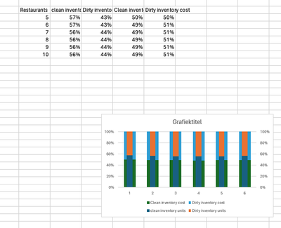
I would love to get to bars next to each with one including clean inventory vs dirty inventory in units and one clean inventory vs dirty inventory in costs. So that for every number on x-axis there are 2 bars next to each other. This is what I got so far: The two bars are behind each other and I am working with two y-axis even though they are the same? Someone any tips how I get them next to each other? Thank you!
Hi, I would love to get to bars next to each with one including clean inventory vs dirty inventory in units and one clean inventory vs dirty inventory in costs. So that for every number on x-axis there are 2 bars next to each other. This is what I got so far: The two bars are behind each other and I am working with two y-axis even though they are the same? Someone any tips how I get them next to each other? Thank you! Read More


