

Category: News

Join tech enthusiasts at MS Build ’24: Exploring AI, Machine Learning, Azure, and More!
Hello and welcome to my first blog post! I’m Suniti, an enthusiastic Microsoft Learn Student Ambassador, pursing graduation in the field of Data Science. Today, I’m super excited to discuss the upcoming MS Build’24 event with all of you!
Join us in celebrating the 14th edition of MS Build, as Microsoft draws closer to celebrating its 50 Years of establishment next year, filled with innovation and challenges. So, let’s have a look at what’s in for you in this exciting event!
What’s the buzz About MS Build?
Ready to immerse yourself in all things AI, machine learning, Azure, Generative AI, and beyond? I am!
MS Build is an annual 3 day-long, conference organised by Microsoft. This year’s is all about “ How AI Will Shape Your Future?”. Microsoft Build promises you get an exclusive peek into the latest AI innovations. This year the schedule for the event is May 21 -24, 2024 for in-person and May 21 – 23, 2024 for online attendees.
What to Expect:
Brief of the most recent changes in Azure AI Services, Microsoft Fabric, .Net, and the Azure OpenAI Service.
Keynotes, live demos, and breakout sessions that will boost your minds from the experts of Microsoft.
Exclusive insights into emerging technologies from Microsoft.
Event swag and digital swag.
Microsoft Cloud Skills Challenge to enhance your learning journey.
Get a chance to connect with Industry experts and get answers to your questions.
Meet the Keynote Speakers:
Satya Nadella, CEO of Microsoft
Rajesh Jha, EVP
Scott Guthrie, EVP Cloud + AI
And many more!
Recapping MS Build 2023
Were you there in MS Build’23? If No, here is a recap of what new was introduced last year.
Window’s Copilot – Learn more
Bringing Bing to ChagGPT
Copilot and Plugins – Learn more
Helping Solve Humanity’s Greatest Challenges with AI Tools
Jugalbandi Chat Bot
Get Started with AI on Microsoft Azure – Learn more
These were the most liked and popular among developers. If you want to explore more, what was there for you. in MS Build’23. Click Here
The History of MS Build
Since its inception in 2011, Microsoft Build has been a beacon of innovation and collaboration. From Anaheim to Seattle, this annual gathering has evolved into a platform, uniting developers and technologists from every corner of the world.
How It Starts:
The conference is organized in a hybrid mode.
In-person: Microsoft Build will be held at the Seattle, corporate headquarters of Microsoft Corporation. It will cost you $1,825 to attend the session offline.
Online: Everyone around the world can attend the session, once you register you will receive a digital attendee pass and an email for confirmation.
The Keynote on the first day was led by the Microsoft CEO Satya Nadella addressing the press and developers. Then, there are breakout sessions led by Microsoft’s Minds, where you can learn new technologies. Thousands of developers from all over the world will attend, so it’s a great chance to network and make some connections too.
| Register now at Microsoft Build 2024
Building a Brighter Future
Microsoft always fosters a welcoming environment for all. Building AI solutions following Responsible AI principles and the opportunity to learn from and connect with diverse students and professionals from various countries, religions, genders, and races. Having been part of the community since April ’23, I’ve had as an MLSA. This experience has been enriching, allowing me to engage in a wide range of activities, from learning and teaching to sharing ideas and collaborating on projects.
So, are you ready to embark on your journey fuelled with AI? Join, along with me in the conversation at Microsoft Build 2024. See you there!
Resources
MS Build | Scaling Future
Wikipedia | History of MS Build
MS Developers | YouTube
Thanks for diving into the excitement with me! Let’s keep the conversation going as we look forward to Microsoft Build 2024. See you there!
Microsoft Tech Community – Latest Blogs –Read More
Why do I receive “Products Already Installed” when installing MathWorks products?
Why do I receive "Products Already Installed" when installing MathWorks products?Why do I receive "Products Already Installed" when installing MathWorks products? Why do I receive "Products Already Installed" when installing MathWorks products? why do i receive "products already installed" when MATLAB Answers — New Questions
removing quotes from table
Hi,
I have a table with gregorian time that loads as having single quotes around it. This is giving me issues when I want to do table2timetable.
How do I remove the quotes so I can convert to timetable?
Thanks!Hi,
I have a table with gregorian time that loads as having single quotes around it. This is giving me issues when I want to do table2timetable.
How do I remove the quotes so I can convert to timetable?
Thanks! Hi,
I have a table with gregorian time that loads as having single quotes around it. This is giving me issues when I want to do table2timetable.
How do I remove the quotes so I can convert to timetable?
Thanks! removing quotes, timetable MATLAB Answers — New Questions
Warning: Not enough data imported. Attempt to read… (Dicominfo/Dicomdisp)
Hello,
I would like to ask how to solve this issue in matlab, while I am trying to read several dicom images I have got from PACS. Radiant application shows images normally, but Matlab does not recognise the size of them, width and height, and I am getting this warning as well, when i call dicominfo:
The second number of bytes (only read) is the actual size of my picture(.dcm), and however, Matlab attempts to read like 1,3Gb of data, instead the actual size of it which is 12Mb.
Also, when i use dicomdisp i get the following:
I have highlighted where i find the actual size, in that private attribute, and also noticed how there is no location 6182 (it ends at 6170), and there are some more attributes which their size is like 4.3 Gb. Is reading it on IEEE little-endian machine related with my computer or PACS? Could that be the reason? Widh and Height attributes are both in dicomdisp and Radiant (Dicom Viewer Application) shown as WindowWidth/WindowCenter and WL/WW respectively. Therefore, it could be some sort of incompatibility between headers/attributes from one source to another?
Is it something to do with their actual size of my dicom pictures, which is rather too much for my laptop to handle? They are 2k x 4k resolution. So, since my screen doesnt support that resolution, maybe that’s why Matlab open just a blank figure? Still, shouldnt it have been able to read width and height with dicominfo?
In addition to that, in line (63) at dicominfo.m describes some issues about parsing the dicom file and its attributes, but I am not sure if it is related with the previous issue.
Any help would be grateful.Hello,
I would like to ask how to solve this issue in matlab, while I am trying to read several dicom images I have got from PACS. Radiant application shows images normally, but Matlab does not recognise the size of them, width and height, and I am getting this warning as well, when i call dicominfo:
The second number of bytes (only read) is the actual size of my picture(.dcm), and however, Matlab attempts to read like 1,3Gb of data, instead the actual size of it which is 12Mb.
Also, when i use dicomdisp i get the following:
I have highlighted where i find the actual size, in that private attribute, and also noticed how there is no location 6182 (it ends at 6170), and there are some more attributes which their size is like 4.3 Gb. Is reading it on IEEE little-endian machine related with my computer or PACS? Could that be the reason? Widh and Height attributes are both in dicomdisp and Radiant (Dicom Viewer Application) shown as WindowWidth/WindowCenter and WL/WW respectively. Therefore, it could be some sort of incompatibility between headers/attributes from one source to another?
Is it something to do with their actual size of my dicom pictures, which is rather too much for my laptop to handle? They are 2k x 4k resolution. So, since my screen doesnt support that resolution, maybe that’s why Matlab open just a blank figure? Still, shouldnt it have been able to read width and height with dicominfo?
In addition to that, in line (63) at dicominfo.m describes some issues about parsing the dicom file and its attributes, but I am not sure if it is related with the previous issue.
Any help would be grateful. Hello,
I would like to ask how to solve this issue in matlab, while I am trying to read several dicom images I have got from PACS. Radiant application shows images normally, but Matlab does not recognise the size of them, width and height, and I am getting this warning as well, when i call dicominfo:
The second number of bytes (only read) is the actual size of my picture(.dcm), and however, Matlab attempts to read like 1,3Gb of data, instead the actual size of it which is 12Mb.
Also, when i use dicomdisp i get the following:
I have highlighted where i find the actual size, in that private attribute, and also noticed how there is no location 6182 (it ends at 6170), and there are some more attributes which their size is like 4.3 Gb. Is reading it on IEEE little-endian machine related with my computer or PACS? Could that be the reason? Widh and Height attributes are both in dicomdisp and Radiant (Dicom Viewer Application) shown as WindowWidth/WindowCenter and WL/WW respectively. Therefore, it could be some sort of incompatibility between headers/attributes from one source to another?
Is it something to do with their actual size of my dicom pictures, which is rather too much for my laptop to handle? They are 2k x 4k resolution. So, since my screen doesnt support that resolution, maybe that’s why Matlab open just a blank figure? Still, shouldnt it have been able to read width and height with dicominfo?
In addition to that, in line (63) at dicominfo.m describes some issues about parsing the dicom file and its attributes, but I am not sure if it is related with the previous issue.
Any help would be grateful. dicominfo MATLAB Answers — New Questions
error in concatenating cells
Hello Dear,
I have 1×50 cell (ftData728178E.trial) in a struct. Each cell has a 192×2301 double. After I concatenate the cell to make a matrix of 192x2301x50, the matrix turns into nan. I wonder why it is and what the correct way to turn cells into a matrix. Thanks,
ET
ft_epoch = cat(3, ftData728178E.trial{:});Hello Dear,
I have 1×50 cell (ftData728178E.trial) in a struct. Each cell has a 192×2301 double. After I concatenate the cell to make a matrix of 192x2301x50, the matrix turns into nan. I wonder why it is and what the correct way to turn cells into a matrix. Thanks,
ET
ft_epoch = cat(3, ftData728178E.trial{:}); Hello Dear,
I have 1×50 cell (ftData728178E.trial) in a struct. Each cell has a 192×2301 double. After I concatenate the cell to make a matrix of 192x2301x50, the matrix turns into nan. I wonder why it is and what the correct way to turn cells into a matrix. Thanks,
ET
ft_epoch = cat(3, ftData728178E.trial{:}); cell, concatention, matrix MATLAB Answers — New Questions
How to send a message to a specific user
I want to send a message to a specific user from external service using the user ID.
In the sample code, I can use “getPagedInstallations” to loop through all users.
—————————————–
—————————————–
I think this is bad performance.
Is there any other better way?
I want to send a message to a specific user from external service using the user ID. In the sample code, I can use “getPagedInstallations” to loop through all users.—————————————–const pagedData = await notificationApp.notification.getPagedInstallations( pageSize, continuationToken); const installations = pagedData.data;for (const target of installations) { …}—————————————– I think this is bad performance.Is there any other better way? Read More
Unveiling Generative AI Bulk Processing and Ingestion Pattern
Generative and embeddings models have taken the world by storm in recent years, producing high-quality natural language responses for various tasks and domains. Organizations, start-ups, and innovators across the world have been exploring the applications of this capability through prototyping, small-scale proof of concepts, and influencing text outputs through prompt engineering. As they gain more understanding of generative AI concepts such as context length, tokens, embeddings, and attention, as well as methods to avoid hallucinations, they discover new use cases and opportunities for leveraging this technology. One of the most popular and widely applicable use cases is search-based answer generation, which can enhance the user experience and satisfaction for any industry that relies on information retrieval and query answering.
This technical blog describes a pattern for bulk processing and ingestion with generative AI, which can help organizations grow their generative AI solutions from prototype and proof of concept phases to pilot and production workloads. The described bulk processing and ingestion pattern leverages the parallel and distributed computing capabilities of Azure platform to generate and store large volumes of natural language responses based on a given set of PDF documents. The blog also provides a walkthrough of the sample code made available on the Github repository, which implements this pattern using Azure OpenAI, Azure Functions, Azure Queue Storage, Azure Document Intelligence, Azure CosmosDB and potentially Azure AI Search. The code can be easily customized and adapted to different generative AI models and use cases, such as knowledgebase population for search-based answer generation.
Architecture Overview
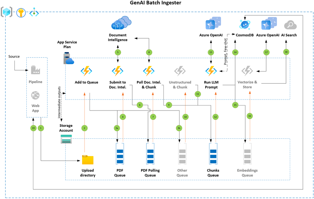
Figure 1: Key components and execution flow
The solution takes advantage of the event-driven processing paradigm. As soon as the input documents are uploaded to a designated Azure Storage location, they trigger an event that invokes Azure Functions written in Python to extract text from the documents. The extracted text is then split into smaller segments of text (based on a configurable token count value) and concatenated into larger segments (also configurable). This approach allows for flexibility in generating text at different levels of granularity, depending on the context length supported by the large language models (LLMs).
The concatenated segments are then processed in parallel, making API calls to one or more Azure OpenAI endpoints to apply a default prompt predefined in the Azure CosmosDB database. The prompt to be applied can be customized at the document level by adding its id to the blob metadata. If the document blob has a prompt_id metadata tag that points to a user-defined prompt value available in the Azure CosmosDB, then that prompt will be used. Otherwise, the default prompt (also configurable) will be applied. All intermediate outputs are stored in Azure Storage for traceability back to the source document. The text can also be vectorized and indexed by an AI Search service by cloning and modifying the Run LLM Prompt function. The vectorization step is not implemented in sample code.
Code components from different publicly available accelerators made by internal teams are reused in this solution. We thank them for their work.
Flow Details
Incremental offload (Step 1)
When processing large sets of documents, it is a best practice to split the work in small batches of documents and have them processed one set of documents at a time. You can build a simple pipeline that fetches and offloads the documents batch by batch into designated storage account container. Next batch can be added upon successful completion of previous. Alternatively, there could be use cases where you can offer upload functionality directly to users through a web application.
Queued for processing (Steps 2 and 3a)
Each arriving document triggers the Azure Function that queues the document to be submitted to Document Intelligence endpoint. The code implementation of this pattern currently supports processing of PDF files and can be easily extended to handle other file types.
Submitted to Document Intelligence (Steps 4, 5 and 6)
As the next step, the BLOB URL of the document is appended with a SAS token and submitted to Document Intelligence endpoint. The Document Intelligence API returns a unique identifier upon accepting the document for extracting the text. This unique identifier is passed to the next queue to keep polling the Document Intelligence endpoint until it has processed the document.
Verify that Document Intelligence processing is completed and chunk the text (Steps 7, 8 and 9)
The time to analyze a document depends on the size (for example, number of pages) and associated content on each page. This step keeps polling Document Intelligence until the status code 200 is received. Otherwise requeue the message to trigger a new instance of the check without looping inside the code. This is a powerful feature that queues offer. Once the status code 200 is received, the text response is chunked and details of the merged chunks are passed to the next que to apply prompt (or vectorize and ingest into AI Search) or any other task that you would like to accomplish as part of the flow.
Figure 2: Chunks queue message structure
Apply LLM prompt (Steps 12, 13, 14)
Each merged chunk is prefixed with system message (configurable) and default (or user defined) prompt retrieved from the Azure CosmosDB which acts as a metadata and information logging database. The updated prompt is passed to Azure OpenAI chat completion endpoint. The response from Azure OpenAI endpoint is saved into both Azure Storage and Azure CosmosDB. In case your use case requires few shot examples to be passed per prompt, you may store these few shot examples in the Azure CosmosDB and fetch them dynamically along with the prompt to be given to a large language model.
(Alternatively) Vectorize and ingest into AI Search (Steps 15, 16, 17, 18)
You could easily clone the Apply LLM prompt function to achieve embedding generation for the merged chunk and store each chunk as an AI Search document along with reference to the source document.
Intermediate outputs
Saving the outputs produced by each flow step is a best practice when a flow is broken into multiple steps. These outputs can be handy to re-run part of the flow by rehydrating the storage queue with messages. The provided sample code that implements this pattern stores all intermediate outputs in the Azure Storage.
Figure 3: After text is extracted by Document Intelligence API
Figure 4: Chunks are created
Figure 5: Prompt output
Addressing request throttling
The sample code in Github demonstrates use of multiple (you may also use a single) endpoints to distributes the request across Azure Document Intelligence and Azure OpenAI endpoints. Please see below additional considerations for mitigating the request throttling.
Azure Document Intelligence
Implement retry logic in your application.
If you find that you’re being throttled on the number of POST requests, consider adding a delay between the requests.
Increase the workload gradually. Avoid sharp changes.
Create a support request to increase transactions per second (TPS) limit.
Azure OpenAI
Implement client-side retry logic to wait the retry-after-ms time and retry.
Consider redirecting the traffic to other models, deployments.
Move quota from another deployment, if necessary.
Please review references section of this article for additional information links to product documentation.
Monitoring the progress
A detailed process log is maintained in the Azure CosmosDB at the granularity of each merged chunk. You can review the process logs and stay on top of the processing status by using NoSQL API for Azure CosmosDB. Sample queries are show below, you may write additional queries. For instance chunks that may have encountered error or were skipped and the supporting error message to perform further investigations.
Figure 6: View chunk progress log
Figure 7: LLM output saved in the Azure CosmosDB
Execution Times
Please see below the execution time for the test dataset and setup combinations in our sandbox environment. With each test we added more files and increased the infrastructure configuration to confirm the scaling aspect of this pattern. These numbers may vary based on your workload and implementation details – whether you are applying an LLM prompt to chunks or generating embeddings or doing both, chunk size, the output token size you have selected, the LLM model, etc.
References
GitHub Code sample – GenAI-Batch-Ingester
Azure OpenAI Service REST API reference
Azure OpenAI – Staying within rate limits
Azure OpenAI – PTU
Document Intelligence API
Document Intelligence – Mitigating throttling
Azure Queue storage trigger and bindings for Azure Functions
Microsoft Tech Community – Latest Blogs –Read More
Setting common color maps for categorical images with no ordinal information in the categorical labels
I’m trying to create a common colormap from two different categorical images that are segmentations of brain regions. The labels in "oldsegvis" are an entirely contained subset of the labels in "newsegvis". I’m expecting the same label value (e.g. newseg = 100, oldseg = 100) to return the same color, however, that is not the output behavior I’m observing. I’ve confirmed by looking at the values in the output newsegvis and oldsegvis arrays and by using "Data Tips" that the same values are being assigned different colors. Additionally, in the visualization of the "newsegvis" array, different values are being assigned the same color, which I’ve also confirmed with "Data Tips", even though the number of colors and the number of unique label values are the same. A code snippet is pasted below; I’m sure there’s something simple I’m missing, but would be very appreciative if someone could point it out to me. Thanks!
%% Visualize segmentations
%select section (transverse plane)
newsegvis = squeeze(newvol(:,:,100));
oldsegvis = squeeze(oldvol(:,:,100));
%set colormaps (new segmentations have all old segmentation labels plus
%additional labels)
newsegs = unique(newsegvis);
oldsegs = unique(oldsegvis);
cmap_ov = [0 0 0;rand(length(newsegs)-1,3)];
cmap_orig = cmap_ov(1:length(oldsegs),:);
%visualize segmentations
figure; imagesc(newsegvis); colormap(cmap_ov);
figure; imagesc(oldsegvis); colormap(cmap_orig);I’m trying to create a common colormap from two different categorical images that are segmentations of brain regions. The labels in "oldsegvis" are an entirely contained subset of the labels in "newsegvis". I’m expecting the same label value (e.g. newseg = 100, oldseg = 100) to return the same color, however, that is not the output behavior I’m observing. I’ve confirmed by looking at the values in the output newsegvis and oldsegvis arrays and by using "Data Tips" that the same values are being assigned different colors. Additionally, in the visualization of the "newsegvis" array, different values are being assigned the same color, which I’ve also confirmed with "Data Tips", even though the number of colors and the number of unique label values are the same. A code snippet is pasted below; I’m sure there’s something simple I’m missing, but would be very appreciative if someone could point it out to me. Thanks!
%% Visualize segmentations
%select section (transverse plane)
newsegvis = squeeze(newvol(:,:,100));
oldsegvis = squeeze(oldvol(:,:,100));
%set colormaps (new segmentations have all old segmentation labels plus
%additional labels)
newsegs = unique(newsegvis);
oldsegs = unique(oldsegvis);
cmap_ov = [0 0 0;rand(length(newsegs)-1,3)];
cmap_orig = cmap_ov(1:length(oldsegs),:);
%visualize segmentations
figure; imagesc(newsegvis); colormap(cmap_ov);
figure; imagesc(oldsegvis); colormap(cmap_orig); I’m trying to create a common colormap from two different categorical images that are segmentations of brain regions. The labels in "oldsegvis" are an entirely contained subset of the labels in "newsegvis". I’m expecting the same label value (e.g. newseg = 100, oldseg = 100) to return the same color, however, that is not the output behavior I’m observing. I’ve confirmed by looking at the values in the output newsegvis and oldsegvis arrays and by using "Data Tips" that the same values are being assigned different colors. Additionally, in the visualization of the "newsegvis" array, different values are being assigned the same color, which I’ve also confirmed with "Data Tips", even though the number of colors and the number of unique label values are the same. A code snippet is pasted below; I’m sure there’s something simple I’m missing, but would be very appreciative if someone could point it out to me. Thanks!
%% Visualize segmentations
%select section (transverse plane)
newsegvis = squeeze(newvol(:,:,100));
oldsegvis = squeeze(oldvol(:,:,100));
%set colormaps (new segmentations have all old segmentation labels plus
%additional labels)
newsegs = unique(newsegvis);
oldsegs = unique(oldsegvis);
cmap_ov = [0 0 0;rand(length(newsegs)-1,3)];
cmap_orig = cmap_ov(1:length(oldsegs),:);
%visualize segmentations
figure; imagesc(newsegvis); colormap(cmap_ov);
figure; imagesc(oldsegvis); colormap(cmap_orig); colormap, imagesc MATLAB Answers — New Questions
Support for NVIDIA RTX A1000
I am evaluating if a Dell laptop with an NVIDIA RTX A1000 graphics card can take advantage of the GPU accleration in Matlab. The NVIDIA site does not list the ‘compute capability’ of the RTX A1000 in the table of current or legacy graphic cards.I am evaluating if a Dell laptop with an NVIDIA RTX A1000 graphics card can take advantage of the GPU accleration in Matlab. The NVIDIA site does not list the ‘compute capability’ of the RTX A1000 in the table of current or legacy graphic cards. I am evaluating if a Dell laptop with an NVIDIA RTX A1000 graphics card can take advantage of the GPU accleration in Matlab. The NVIDIA site does not list the ‘compute capability’ of the RTX A1000 in the table of current or legacy graphic cards. nvidia rtx a1000 MATLAB Answers — New Questions
What does it mean “/Multiple” after variable name in *.mat file?
I have *.mat files exported by Bruker Opus program. When I select these files Matlab lists the variables contained in that file. However, after each variable name there is a /Multiple note, (see figure).
When I click on the file it does not load anything.
What does it mean the "/Multiple"? How to load these files?I have *.mat files exported by Bruker Opus program. When I select these files Matlab lists the variables contained in that file. However, after each variable name there is a /Multiple note, (see figure).
When I click on the file it does not load anything.
What does it mean the "/Multiple"? How to load these files? I have *.mat files exported by Bruker Opus program. When I select these files Matlab lists the variables contained in that file. However, after each variable name there is a /Multiple note, (see figure).
When I click on the file it does not load anything.
What does it mean the "/Multiple"? How to load these files? bruker, opus, mat files, /multiple flag? MATLAB Answers — New Questions
Azure IoT hub & edge gateways
Hi,
We are evaluating azure IoT for implementing IoT pipeline for one of our customer.
We are looking for latest case study and implementation references, also we have few queries. Please help us with references and documentation.
1. Do we have any recent case study & Business cases references using the Azure IoT hub/edge?
2. Any sample case studies for implementing the IoT edge as gateways for protocol translation?
3. Do we have any recent reference for SDKs for Java/Python to build the Custom modules for translational gateways handling multiple protocol translations? GitHub we came across were atleast 2-4 years old.
4. Where can we find the details on defining the device and connect them to the IoT Edge gateway?
5. Do we have latest documentation on the IoT Edge Windows deployment?
Thanks,
Hi,We are evaluating azure IoT for implementing IoT pipeline for one of our customer. We are looking for latest case study and implementation references, also we have few queries. Please help us with references and documentation.1. Do we have any recent case study & Business cases references using the Azure IoT hub/edge?2. Any sample case studies for implementing the IoT edge as gateways for protocol translation?3. Do we have any recent reference for SDKs for Java/Python to build the Custom modules for translational gateways handling multiple protocol translations? GitHub we came across were atleast 2-4 years old.4. Where can we find the details on defining the device and connect them to the IoT Edge gateway?5. Do we have latest documentation on the IoT Edge Windows deployment? Thanks, Read More
Looking value in another sheet and returns the ID
Hi All,
I have excel file in that i have 2 sheets S1 (orange) & S2 (blue). I have CID column in S2 and I want to check D column value of S2 in C column of S1 and then i want to return the ID in CID column
for example, I have 5 entries in S2 sheet
BadakhshanAfghanistanBadakhshanAfghanistanBadakhshanAfghanistanBadakhshanAfghanistanBadakhshanAfghanistanBadakhshanAfghanistan
and in S1 i have this
CONCAT2ID
BadakhshanAfghanistan1
So I want the result in S2 to be
CONCAT1 CID
BadakhshanAfghanistan1BadakhshanAfghanistan1BadakhshanAfghanistan1BadakhshanAfghanistan1BadakhshanAfghanistan1BadakhshanAfghanistan1
i have added excel sheet as well for your reference. Thanks 🙂
Hi All, I have excel file in that i have 2 sheets S1 (orange) & S2 (blue). I have CID column in S2 and I want to check D column value of S2 in C column of S1 and then i want to return the ID in CID column for example, I have 5 entries in S2 sheetBadakhshanAfghanistanBadakhshanAfghanistanBadakhshanAfghanistanBadakhshanAfghanistanBadakhshanAfghanistanBadakhshanAfghanistan and in S1 i have this CONCAT2IDBadakhshanAfghanistan1 So I want the result in S2 to beCONCAT1 CIDBadakhshanAfghanistan1BadakhshanAfghanistan1BadakhshanAfghanistan1BadakhshanAfghanistan1BadakhshanAfghanistan1BadakhshanAfghanistan1 i have added excel sheet as well for your reference. Thanks 🙂 Read More
Start and Wait for approval
I want to utilize the functionality provided by the Microsoft Graph API to initiate and await approval for timesheets stored in SharePoint. Could someone please assist me in understanding the process for implementing this?
I want to utilize the functionality provided by the Microsoft Graph API to initiate and await approval for timesheets stored in SharePoint. Could someone please assist me in understanding the process for implementing this? Read More
Update 2403 for Microsoft Configuration Manager current branch is now available.
Update 2403 for Configuration Manager current branch is available as an in-console update. Apply this update on sites that run version 2211 or later. When installing a new site, it will also be available as a baseline version soon after general availability. This article summarizes the changes and new features in Configuration Manager, version 2403.
Site infrastructure
Starting Configuration Manager version 2403, Microsoft Azure Active Directory is renamed to Microsoft Entra ID within Configuration Manager.
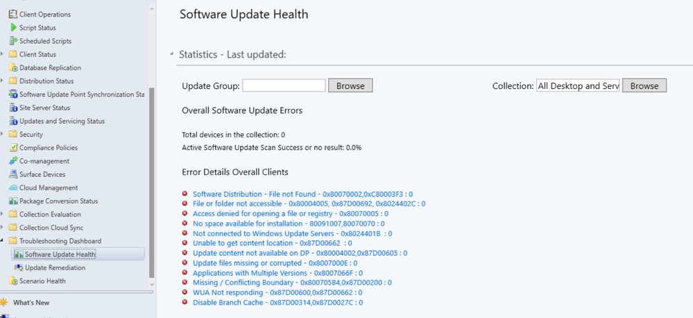
Automated diagnostic Dashboard for Software Update Issues
A new dashboard is added to the console under monitoring workspace, which shows the diagnosis of the software update issues in your environment this feature can easily identify any issues related to software updates. You can fix software update issues based on troubleshooting documentations.
Special credit to Shankar Subramanian and Smita Jadhav for their details and troubleshooting notes.
For more information, see Software update health dashboard.
Users can now use the global search box in CM console, which streamlines the search experience and centralizes access to information. This feature enhances the overall usability, productivity and effectiveness of CM. Users no longer need to navigate through multiple nodes or sections/ folders to find information they require, saving valuable time and effort.
For more information, see Improvements to console search.
You can now organize scripts by using folders. This change allows for better categorization and management of scripts. Full Administrator and Operations Administrator roles can manage the folders.
For more information, see Folder support for scripts.
HTTPS or Enhanced HTTP should be enabled for client communication from this version of Configuration Manager
HTTP-only communication is deprecated, and support is removed from this version of Configuration Manager. Enable HTTPS or Enhanced HTTP for client communication.
For more information, see Enable site system roles for HTTPS or Enhanced HTTP. and Deprecated features
Windows Server 2012/2012 R2 operating system site system roles are not supported from this version of Configuration Manager
Starting 2403, Windows Server 2012/2012 R2 operating system site system roles aren’t supported in any CB releases. Clients with extended support (ESU) will continue to support.
For more information, see Supported-operating-systems-for-site-system-servers.
Any configured Resource access profiles and deployments block Configuration manager upgrade. Consider deleting them and moving the co-management workload for Resource Access (if co-managed) to Intune.
For more information, see FAQ and Resource access policies are no longer supported.
A new parameter SoftwareUpdateO365Language is now added to PowerShell Save-CMSoftwareUpdate cmdlet. Customers now don’t have to check a specific language in the SUP Properties (causing a metadata download for that language for all updates).
PowerShell Commandlet: Save-CMSoftwareUpdate – SoftwareUpdateO365Language <language name> (<region name>)”
Note
Languages need to be in O365 format to be consistent with Admin Console UI. E.g. “Hungarian (Hungary)”.
Configuration Manager operating system deployment support is now added on Windows 11 ARM 64 devices. Currently Importing and customizing Arm 64 boot images, Wipe and load TS, Media creation TS, WDS PXE for Arm 64 and CMPivot is supported.
Administrators while deploying the “Install Software Package” via Dynamic variable with “Continue on error” unchecked to clients, will not be notified with task sequence failures even if package versions on the distribution point are updated.
For more information, see Options for Install Application.
The option to upgrade Configuration Manager 2403 is blocked if you’re running cloud management gateway V1 (CMG) as a cloud service (classic). All CMG deployments should use a virtual machine scale set.
For more information, see Check for a cloud management gateway (CMG) as a cloud service (classic).
Learn about support changes before they’re implemented in removed and deprecated items.
System Center Update Publisher (SCUP) and integration with ConfigMgr planned end of support Jan 2024.
For more information, see Removed and deprecated features for Configuration Manager.
This release includes the following improvements to BitLocker:
Starting in this release, this feature ensures proper verification of key escrow and prevents message drops. We now validate whether the key is successfully escrowed to the database, and only on successful escrow we add the key protector.
This feature now prevents a potential data loss scenario where BitLocker is protecting the volumes with keys that are never backed up to the database, in any failures to escrow happens.
For more information on BitLocker management, see Deploy BitLocker management. and Plan for BitLocker management..
From this version of Configuration Manager, the Windows 11 readiness dashboard shows charts for Windows 23H2.
Defender Exploit Guards policy for controlled folder now accepts regex in the file path for apps. For example, [C:FolderSubfolderapp?.exe] [C:Folder1Sub*Name]
At this time, version 2403 is released for the early update ring. To install this update, you need to opt in. For more information, see Early update ring.
Thank you,
The Configuration Manager team
Additional resources:
What’s New in Configuration Manager
Documentation for Configuration Manager
Microsoft Configuration Manager announcement
Microsoft Configuration Manager vision statement
Evaluate Configuration Manager in a lab
Upgrade to Configuration Manager
Configuration Manager Forums
Configuration Manager Support
Report an issue
Provide suggestions
Microsoft Tech Community – Latest Blogs –Read More
Wired for Hybrid – What’s New in Azure Networking – April 2024 edition
Hello Folks,
Azure Networking is the foundation of your infrastructure in Azure. Each month we bring you an update on What’s new in Azure Networking.
In this blog post, we’ll cover what’s new with Azure Networking in April 2024. In this blog post, we will cover the following announcements and how they can help you.
Listener TLS certificates management in the Azure portal
Application Gateway for Containers
Application Gateway (v2) IPv6 support
Microsoft open sources Retina: A cloud-native container networking observability platform
Azure Virtual Network encryption now in additional regions
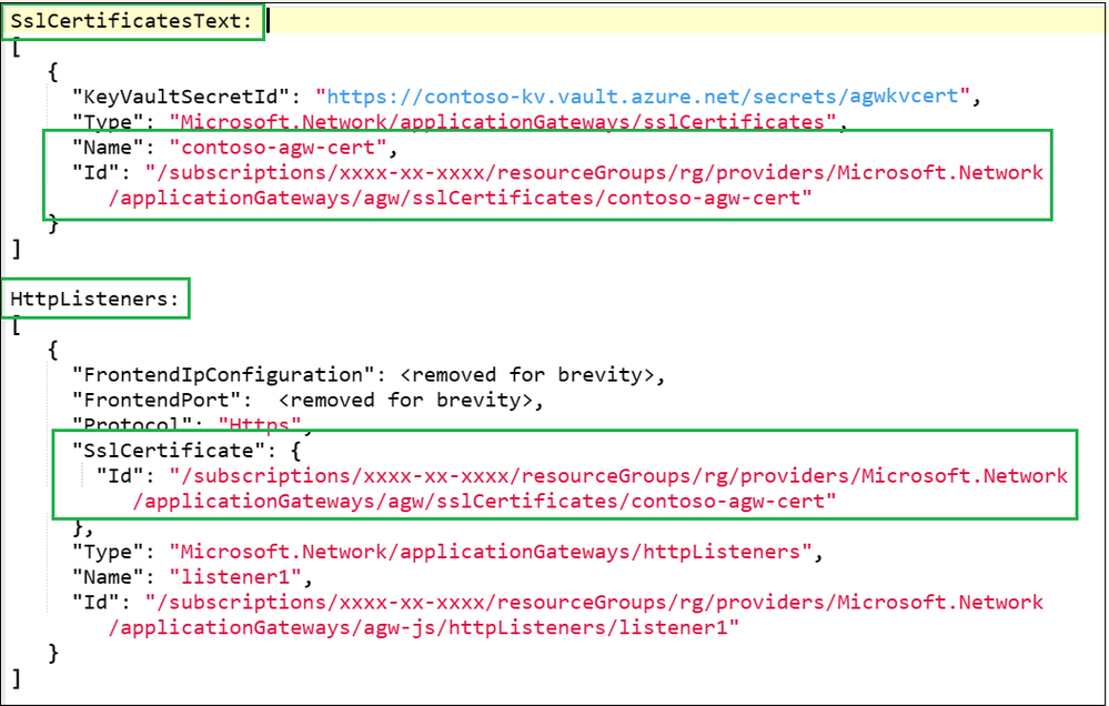
Listener TLS certificates management in the Azure portal
With this GA release, you can more easily manage TLS certificates for your Application Gateway workloads in the Azure Portal.
The Azure Application Gateway is a proxy load balancer that operates at Layer-7, the application layer of the OSI model. Now it supports Layer-4 proxy with TCP and TLS protocols as well. This provides scalable, highly available, and secure application delivery. One of its key features is the ability to secure client traffic through TLS termination, which requires TLS server certificates for listeners. For large gateways with multiple HTTPS or TLS listeners, this means managing multiple .PFX certificates.
For certificate management in the portal, you can list and manage your certificates.
Expiry
Common Name
Thumbprint
Issuer Name
Each certificate includes the following details for quick identification:
Managing certificates in any organization can be a challenge. This is a great addition for reducing friction for admins responsible for secure workloads utilizing certificates.
References:
Application Gateway TCP/TLS proxy overview (Preview)
Listener TLS certificate management in Application Gateway
Quickstart: Direct web traffic using the portal – Azure Application Gateway
TLS termination with Azure Key Vault certificates
General availability: Application Gateway for Containers
Application Gateway for Containers is GA. With this release, you get application (layer 7) load balancing and dynamic traffic management capabilities for workloads running in a Kubernetes cluster.
Application Gateway for Containers is the evolution of the Application Gateway Ingress Controller (AGIC), a Kubernetes application that enables Azure Kubernetes Service (AKS) customers to use Azure’s native Application Gateway application load-balancer. In its current form, AGIC monitors a subset of Kubernetes Resources for changes and applies them to the Application Gateway, utilizing Azure Resource Manager (ARM).
Features – Public preview and GA has added support for Custom Health Probes, URL Redirect, URL / Header Rewrite.
Controller High Availability – Have peace of mind if a node goes down, changes within your cluster will continue to be propagated to the network.
Gateway API v1 – Bring the familiarity and role based access control provided by Gateway API to your network configuration.
Additional Region Availability – Take advantage of Application Gateway for Containers in a region closest to you.
SLA for Production Workloads – Feel confident in running your production workloads with Application Gateway for Containers.
References:
What is Application Gateway for Containers?
Application Gateway for Containers components
Quickstart: Deploy Application Gateway for Containers ALB Controller
What is Azure Application Gateway Ingress Controller?
Application Gateway (v2) IPv6 support
We are announcing that IPv6 support for Azure Application Gateway (v2) is now generally available.
With the addition of IPv6 support, you can take advantage of the increased address space and improved routing efficiency that IPv6 provides. This is especially important for customers who are running out of IPv4 addresses or who need to support IPv6 clients.
To get started with IPv6 support for Azure Application Gateway (v2), simply create a new Application Gateway and select both IPv4 and IPv6 frontends during the creation process. You can also find more information about IPv6 support in our documentation.
References:
Configure Application Gateway with a frontend public IPv6 address using the Azure portal
What is Azure Application Gateway v2?
Microsoft open sources Retina: A cloud-native container networking observability platform
Retina is an open-source Kubernetes Network Observability platform designed to assist with DevOps, SecOps, and compliance use cases. It acts as a centralized hub for monitoring the health, security, and performance of applications and networks within Kubernetes clusters. The platform caters to Cluster Network Administrators, Cluster Security Administrators, and DevOps Engineers.
Provides actionable network insights for cloud-native applications: Retina offers users a way to see how their containerized microservices interact on the network, helping them troubleshoot issues like latency, packet drops and many more.
Non-intrusive and easy to use: Retina works with existing applications without requiring any code changes and provides users with simple ways to observe and troubleshoot network issues.
Supports diverse environments: Designed to be adaptable, Retina works seamlessly with any CNI’s (container network interface), OS, or cloud provider, making it a valuable tool across different environments.
Resources:
Introduction to Retina
Microsoft open sources Retina: Announcement
Azure Virtual Network encryption now in additional regions
Whenever Azure customer traffic moves between datacenters, Microsoft applies a data-link layer encryption method using the IEEE 802.1AE MAC Security Standards (MACsec). This encryption is implemented to secure the traffic outside physical boundaries not controlled by Microsoft or on behalf of Microsoft. This method is applied from point-to-point across the underlying network hardware. Virtual network encryption enables you to encrypt traffic between Virtual Machines and Virtual Machines Scale Sets within the same virtual network. It also encrypts traffic between regionally and globally peered virtual networks. Virtual network encryption enhances existing encryption in transit capabilities in Azure.
With Virtual Network encryption, customers can enable encryption of traffic between Virtual Machines and Virtual Machines Scale Sets within the same virtual network and between regionally and globally peered virtual networks. This new feature enhances the existing encryption in transit capabilities in Azure.
Azure Virtual Network encryption is available in the following additional regions:
West Us
West US 2
East US 2
US East
Europe North
Europe West
France Central
India Central
UAE North
East Asia
Japan West
Japan East
Resources:
What is Azure Virtual Network?
What is Azure Virtual Network encryption?
That’s it for this month.
Cheers
Pierre
Microsoft Tech Community – Latest Blogs –Read More
Using MATLAB to do Numeric Calculus
So I am culminating all of my newfound knowledge to solve and show a simple calculus problem. However I am running into issues…
Given: A piecewise function where v(t)=70t @ t<=20s & 1596.2-9.81t @ 20<t<t_max <—(eq 1)
Also given: s(t)=35t^2+7620 @ t<=20s & 1596.2t-4.905t^2-8342 @ 20<t<=t_max <—(eq 2)
Find: If aircraft ignites its engines at t=0s and accelerates vertically, there is only enough fuel for an engine burn of 20 seconds. At which time will the ship become a projectile? Find value of t_max. Plot the crafts velocity vs. t, (eq 1). Plot the crafts altitude vs. t, (eq 2).
My Solution:
%% Finding Value of tmax
% Finding tmax and rounding it to the nearest whole number
%%
tmaxr=roots([-9.81, 1596.2]);
tmax=ceil(tmaxr);
%% Plotting Equation 1
% Creating Figure 1 from Equation 1
%%
t=0:0.1:tmax;
v=zeros(size(t));
for N=1:length(t)
if t(N)<=20
v(N)=70*t(N);
else
v(N)=1596.2-9.81*t(N); % Only valid for t > 20 seconds
end
end
figure(1)
plot(t,v)
xlabel(‘Time (s)’)
ylabel(‘Velocity (m/s)’)
title(‘Velocity vs. Time’)
%% Plotting Equation 2
% Creating Figure 2 from Equation 2
%%
t=0:0.1:tmax;
s=zeros(size(t));
for N=1:length(t)
if t(N)<=20
s(N)=35.*t(N).^2+7620;
else
s(N)=1596.2.*t(N)-4.905.*t(N).^2-8342;
end
end
figure(2)
plot(t,s)
xlabel(‘Time (s)’)
ylabel(‘Altitude (m)’)
title(‘Position vs. Time’)
Issue: So I have found t_max, plotted the velocity but it looks funky, and also tried to plot my altitide but not sure if it’s faultless.
P.s. Sorry for the formatting, there’s no easy way to type piecewise functions that I know of.So I am culminating all of my newfound knowledge to solve and show a simple calculus problem. However I am running into issues…
Given: A piecewise function where v(t)=70t @ t<=20s & 1596.2-9.81t @ 20<t<t_max <—(eq 1)
Also given: s(t)=35t^2+7620 @ t<=20s & 1596.2t-4.905t^2-8342 @ 20<t<=t_max <—(eq 2)
Find: If aircraft ignites its engines at t=0s and accelerates vertically, there is only enough fuel for an engine burn of 20 seconds. At which time will the ship become a projectile? Find value of t_max. Plot the crafts velocity vs. t, (eq 1). Plot the crafts altitude vs. t, (eq 2).
My Solution:
%% Finding Value of tmax
% Finding tmax and rounding it to the nearest whole number
%%
tmaxr=roots([-9.81, 1596.2]);
tmax=ceil(tmaxr);
%% Plotting Equation 1
% Creating Figure 1 from Equation 1
%%
t=0:0.1:tmax;
v=zeros(size(t));
for N=1:length(t)
if t(N)<=20
v(N)=70*t(N);
else
v(N)=1596.2-9.81*t(N); % Only valid for t > 20 seconds
end
end
figure(1)
plot(t,v)
xlabel(‘Time (s)’)
ylabel(‘Velocity (m/s)’)
title(‘Velocity vs. Time’)
%% Plotting Equation 2
% Creating Figure 2 from Equation 2
%%
t=0:0.1:tmax;
s=zeros(size(t));
for N=1:length(t)
if t(N)<=20
s(N)=35.*t(N).^2+7620;
else
s(N)=1596.2.*t(N)-4.905.*t(N).^2-8342;
end
end
figure(2)
plot(t,s)
xlabel(‘Time (s)’)
ylabel(‘Altitude (m)’)
title(‘Position vs. Time’)
Issue: So I have found t_max, plotted the velocity but it looks funky, and also tried to plot my altitide but not sure if it’s faultless.
P.s. Sorry for the formatting, there’s no easy way to type piecewise functions that I know of. So I am culminating all of my newfound knowledge to solve and show a simple calculus problem. However I am running into issues…
Given: A piecewise function where v(t)=70t @ t<=20s & 1596.2-9.81t @ 20<t<t_max <—(eq 1)
Also given: s(t)=35t^2+7620 @ t<=20s & 1596.2t-4.905t^2-8342 @ 20<t<=t_max <—(eq 2)
Find: If aircraft ignites its engines at t=0s and accelerates vertically, there is only enough fuel for an engine burn of 20 seconds. At which time will the ship become a projectile? Find value of t_max. Plot the crafts velocity vs. t, (eq 1). Plot the crafts altitude vs. t, (eq 2).
My Solution:
%% Finding Value of tmax
% Finding tmax and rounding it to the nearest whole number
%%
tmaxr=roots([-9.81, 1596.2]);
tmax=ceil(tmaxr);
%% Plotting Equation 1
% Creating Figure 1 from Equation 1
%%
t=0:0.1:tmax;
v=zeros(size(t));
for N=1:length(t)
if t(N)<=20
v(N)=70*t(N);
else
v(N)=1596.2-9.81*t(N); % Only valid for t > 20 seconds
end
end
figure(1)
plot(t,v)
xlabel(‘Time (s)’)
ylabel(‘Velocity (m/s)’)
title(‘Velocity vs. Time’)
%% Plotting Equation 2
% Creating Figure 2 from Equation 2
%%
t=0:0.1:tmax;
s=zeros(size(t));
for N=1:length(t)
if t(N)<=20
s(N)=35.*t(N).^2+7620;
else
s(N)=1596.2.*t(N)-4.905.*t(N).^2-8342;
end
end
figure(2)
plot(t,s)
xlabel(‘Time (s)’)
ylabel(‘Altitude (m)’)
title(‘Position vs. Time’)
Issue: So I have found t_max, plotted the velocity but it looks funky, and also tried to plot my altitide but not sure if it’s faultless.
P.s. Sorry for the formatting, there’s no easy way to type piecewise functions that I know of. calculus, plotting MATLAB Answers — New Questions
Installation of MATLAB in Linux failed
I installed MATLAB at a Linux Debian system, but a problem occurs while starting the programme. I’ll get a graphical interface, but in the terminal the following is displayed:
MATLAB is selecting SOFTWARE OPENGL rendering.
/usr/local/MATLAB/R2017b/bin/glnxa64/../../sys/os/glnxa64/libstdc++.so.6: version `CXXABI_1.3.9′ not found (required by /usr/lib/x86_64-linux-gnu/libproxy.so.1)
Failed to load module: /usr/lib/x86_64-linux-gnu/gio/modules/libgiolibproxy.soI installed MATLAB at a Linux Debian system, but a problem occurs while starting the programme. I’ll get a graphical interface, but in the terminal the following is displayed:
MATLAB is selecting SOFTWARE OPENGL rendering.
/usr/local/MATLAB/R2017b/bin/glnxa64/../../sys/os/glnxa64/libstdc++.so.6: version `CXXABI_1.3.9′ not found (required by /usr/lib/x86_64-linux-gnu/libproxy.so.1)
Failed to load module: /usr/lib/x86_64-linux-gnu/gio/modules/libgiolibproxy.so I installed MATLAB at a Linux Debian system, but a problem occurs while starting the programme. I’ll get a graphical interface, but in the terminal the following is displayed:
MATLAB is selecting SOFTWARE OPENGL rendering.
/usr/local/MATLAB/R2017b/bin/glnxa64/../../sys/os/glnxa64/libstdc++.so.6: version `CXXABI_1.3.9′ not found (required by /usr/lib/x86_64-linux-gnu/libproxy.so.1)
Failed to load module: /usr/lib/x86_64-linux-gnu/gio/modules/libgiolibproxy.so linux installation matlab MATLAB Answers — New Questions
I want to increase the distance, the dimensions of the viewing screen should be such that all the beams are on the screen while the pixel value is fixed.
Hi
Look at this code:
close all; clear; clc
N = 2560;
L = 1e4;
dx = 4e-3;
[x0,y0] = meshgrid((-N/2:N/2-1)*dx);
[xL,yL] = meshgrid((-N/2:N/2-1)*dx);
[fx,fy] = meshgrid((-N/2:N/2-1)/(N*dx));
Ni = 37; % Number of beams
d= 25e-2;
a= pi./3;
xi= [ 0 , – d , – d.*cos(a) ,d.*cos(a),d ,d.*cos(a), -d.*cos(a)…
,-2.*d , -2.*d.*cos(a), 0,2.*d.*cos(a), 2.*d, 2.*d.*cos(a),0 , -2.*d.*cos(a)…
, -d-d.*cos(a), d+d.*cos(a), d+d.*cos(a) , -d-d.*cos(a)…
, 3.*d.*cos(a),3.*d.*cos(a)-d, -3.*d.*cos(a)+d , -3.*d.*cos(a), 2.*d.*cos(a)+d,3.*d.*cos(a)+d…
3.*d,3.*d.*cos(a)+d, 2.*d.*cos(a)+d, 3.*d.*cos(a),3.*d.*cos(a)-d, -3.*d.*cos(a)+d , -3.*d.*cos(a)…
,-2.*d.*cos(a)-d ,-3.*d.*cos(a)-d , – 3.*d ,-2.*d.*cos(a)-d ,-3.*d.*cos(a)-d] ;
yi= [ 0 , 0 , d.*sin(a),d.*sin(a), 0 , -d.*sin(a), -d.*sin(a)…
,0 , 2.*d.*sin(a), 2.*d.*sin(a),2.*d.*sin(a), 0 , – 2.*d.*sin(a), -2.*d.*sin(a)…
, – 2.*d.*sin(a), d.*sin(a),d.*sin(a), -d.*sin(a),-d.*sin(a)…
, 3.*d.*sin(a),3.*d.*sin(a),3.*d.*sin(a),3.*d.*sin(a), 2.*d.*sin(a),d.*sin(a), 0 …
, -d.*sin(a), -2.*d.*sin(a), -3.*d.*sin(a), -3.*d.*sin(a), -3.*d.*sin(a),-3.*d.*sin(a)…
,2.*d.*sin(a), d.*sin(a), 0 , -2.*d.*sin(a), -d.*sin(a)];
w0 = 10e-2;
P = 1e3;
lambda = 1080e-9; k = 2*pi/lambda;
L0= 10; l0= 5e-3;
kL= 2.*pi./L0; kl= 5.92./l0;
Cn2= randi([1 1000],1,60)*1e-16;
Kx = 2.*pi.*fx; Ky = 2.*pi.*fy;
U0= 0*x0;
for idx=1:Ni
Utemp = U0 + sqrt(2.*P./pi)./w0 .* exp(-((x0-xi(idx)).^2+(y0-yi(idx)).^2)./w0.^2);
Utemp(((x0-xi(idx)).^2+(y0-yi(idx)).^2)>w0.^2) = 0;
U0= U0 + Utemp;
end
Ui=U0;
figure(1000)
s = pcolor(x0, y0, abs(Ui));
s.EdgeColor = ‘none’;
title("0^{th} Intenesity screen")
xlabel ‘X [m] ‘
ylabel ‘Y [m] ‘
cbar = colorbar;
cbar.Label.String = ‘Intensity(X, Y, 0) [W/cm^2]’;
ax = gca;
axis square
ax.FontName = ‘Times new roman’;
ax.FontSize = 15;
Ni=60; % Number of page views
for idx = 1:Ni
r0= (0.423 .* k.^2 .* Cn2(idx).*L )^(-3/5);
phi = 0.023*r0.^2^(-3./5)*exp(-((Kx^2 + Ky^2) ./ kl.^2)) .* ((Kx.^2 + Ky.^2 + kL^2) ./ (4*pi^2)).^(-11./6);
sigma= 1./(N*dx).*sqrt(phi);
c = randn(N) + i*randn(N);
random_sigma= c.* sigma;
random_sigma(N./2+1,N./2+1)=0;
phi_xy = real(ifftshift(ifft2(ifftshift(random_sigma)))) / dx^2;
Hf = exp(i*k*L).* exp(-i*pi*lambda*L*(fx.^2+fy.^2));
G = fftshift(fft2(fftshift(Ui))) * dx^2;
Ui = ifftshift(ifft2(ifftshift(G.*Hf))) / dx^2;
Ui = Ui .* exp(1i*phi_xy);
figure(2*idx-1)
s = pcolor(x0, y0, phi_xy);
s.EdgeColor = ‘none’;
title(num2str(idx)+"^{th} phase screen")
xlabel ‘X [m]’
ylabel ‘Y [m]’
cbar = colorbar;
cbar.Label.String = ‘Intensity(X, Y, 0) [W/cm^2]’;
ax = gca;
axis square
ax.FontName = ‘Times new roman’;
ax.FontSize = 15;
figure(2*idx)
s = pcolor(xL, yL, abs(Ui));
title(num2str(idx)+"^{th} Intenesity screen")
s.EdgeColor = ‘none’;
xlabel ‘X [m] ‘
ylabel ‘Y [m] ‘
cbar = colorbar;
cbar.Label.String = ‘Intensity(X, Y, 0) [W/cm^2]’;
ax = gca;
axis square
ax.FontName = ‘Times new roman’;
ax.FontSize = 15;
end
In order to see the result at any desired distance (in this code up to L = 1e 4), I have to change the number of pixels (N) according to the desired distance so that all the beams are on the viewing screen.
Now I want the code to be in such a way that by increasing the distance and keeping the number of pixels (512) constant, the dimensions of the viewing screen can accommodate all the beams.Hi
Look at this code:
close all; clear; clc
N = 2560;
L = 1e4;
dx = 4e-3;
[x0,y0] = meshgrid((-N/2:N/2-1)*dx);
[xL,yL] = meshgrid((-N/2:N/2-1)*dx);
[fx,fy] = meshgrid((-N/2:N/2-1)/(N*dx));
Ni = 37; % Number of beams
d= 25e-2;
a= pi./3;
xi= [ 0 , – d , – d.*cos(a) ,d.*cos(a),d ,d.*cos(a), -d.*cos(a)…
,-2.*d , -2.*d.*cos(a), 0,2.*d.*cos(a), 2.*d, 2.*d.*cos(a),0 , -2.*d.*cos(a)…
, -d-d.*cos(a), d+d.*cos(a), d+d.*cos(a) , -d-d.*cos(a)…
, 3.*d.*cos(a),3.*d.*cos(a)-d, -3.*d.*cos(a)+d , -3.*d.*cos(a), 2.*d.*cos(a)+d,3.*d.*cos(a)+d…
3.*d,3.*d.*cos(a)+d, 2.*d.*cos(a)+d, 3.*d.*cos(a),3.*d.*cos(a)-d, -3.*d.*cos(a)+d , -3.*d.*cos(a)…
,-2.*d.*cos(a)-d ,-3.*d.*cos(a)-d , – 3.*d ,-2.*d.*cos(a)-d ,-3.*d.*cos(a)-d] ;
yi= [ 0 , 0 , d.*sin(a),d.*sin(a), 0 , -d.*sin(a), -d.*sin(a)…
,0 , 2.*d.*sin(a), 2.*d.*sin(a),2.*d.*sin(a), 0 , – 2.*d.*sin(a), -2.*d.*sin(a)…
, – 2.*d.*sin(a), d.*sin(a),d.*sin(a), -d.*sin(a),-d.*sin(a)…
, 3.*d.*sin(a),3.*d.*sin(a),3.*d.*sin(a),3.*d.*sin(a), 2.*d.*sin(a),d.*sin(a), 0 …
, -d.*sin(a), -2.*d.*sin(a), -3.*d.*sin(a), -3.*d.*sin(a), -3.*d.*sin(a),-3.*d.*sin(a)…
,2.*d.*sin(a), d.*sin(a), 0 , -2.*d.*sin(a), -d.*sin(a)];
w0 = 10e-2;
P = 1e3;
lambda = 1080e-9; k = 2*pi/lambda;
L0= 10; l0= 5e-3;
kL= 2.*pi./L0; kl= 5.92./l0;
Cn2= randi([1 1000],1,60)*1e-16;
Kx = 2.*pi.*fx; Ky = 2.*pi.*fy;
U0= 0*x0;
for idx=1:Ni
Utemp = U0 + sqrt(2.*P./pi)./w0 .* exp(-((x0-xi(idx)).^2+(y0-yi(idx)).^2)./w0.^2);
Utemp(((x0-xi(idx)).^2+(y0-yi(idx)).^2)>w0.^2) = 0;
U0= U0 + Utemp;
end
Ui=U0;
figure(1000)
s = pcolor(x0, y0, abs(Ui));
s.EdgeColor = ‘none’;
title("0^{th} Intenesity screen")
xlabel ‘X [m] ‘
ylabel ‘Y [m] ‘
cbar = colorbar;
cbar.Label.String = ‘Intensity(X, Y, 0) [W/cm^2]’;
ax = gca;
axis square
ax.FontName = ‘Times new roman’;
ax.FontSize = 15;
Ni=60; % Number of page views
for idx = 1:Ni
r0= (0.423 .* k.^2 .* Cn2(idx).*L )^(-3/5);
phi = 0.023*r0.^2^(-3./5)*exp(-((Kx^2 + Ky^2) ./ kl.^2)) .* ((Kx.^2 + Ky.^2 + kL^2) ./ (4*pi^2)).^(-11./6);
sigma= 1./(N*dx).*sqrt(phi);
c = randn(N) + i*randn(N);
random_sigma= c.* sigma;
random_sigma(N./2+1,N./2+1)=0;
phi_xy = real(ifftshift(ifft2(ifftshift(random_sigma)))) / dx^2;
Hf = exp(i*k*L).* exp(-i*pi*lambda*L*(fx.^2+fy.^2));
G = fftshift(fft2(fftshift(Ui))) * dx^2;
Ui = ifftshift(ifft2(ifftshift(G.*Hf))) / dx^2;
Ui = Ui .* exp(1i*phi_xy);
figure(2*idx-1)
s = pcolor(x0, y0, phi_xy);
s.EdgeColor = ‘none’;
title(num2str(idx)+"^{th} phase screen")
xlabel ‘X [m]’
ylabel ‘Y [m]’
cbar = colorbar;
cbar.Label.String = ‘Intensity(X, Y, 0) [W/cm^2]’;
ax = gca;
axis square
ax.FontName = ‘Times new roman’;
ax.FontSize = 15;
figure(2*idx)
s = pcolor(xL, yL, abs(Ui));
title(num2str(idx)+"^{th} Intenesity screen")
s.EdgeColor = ‘none’;
xlabel ‘X [m] ‘
ylabel ‘Y [m] ‘
cbar = colorbar;
cbar.Label.String = ‘Intensity(X, Y, 0) [W/cm^2]’;
ax = gca;
axis square
ax.FontName = ‘Times new roman’;
ax.FontSize = 15;
end
In order to see the result at any desired distance (in this code up to L = 1e 4), I have to change the number of pixels (N) according to the desired distance so that all the beams are on the viewing screen.
Now I want the code to be in such a way that by increasing the distance and keeping the number of pixels (512) constant, the dimensions of the viewing screen can accommodate all the beams. Hi
Look at this code:
close all; clear; clc
N = 2560;
L = 1e4;
dx = 4e-3;
[x0,y0] = meshgrid((-N/2:N/2-1)*dx);
[xL,yL] = meshgrid((-N/2:N/2-1)*dx);
[fx,fy] = meshgrid((-N/2:N/2-1)/(N*dx));
Ni = 37; % Number of beams
d= 25e-2;
a= pi./3;
xi= [ 0 , – d , – d.*cos(a) ,d.*cos(a),d ,d.*cos(a), -d.*cos(a)…
,-2.*d , -2.*d.*cos(a), 0,2.*d.*cos(a), 2.*d, 2.*d.*cos(a),0 , -2.*d.*cos(a)…
, -d-d.*cos(a), d+d.*cos(a), d+d.*cos(a) , -d-d.*cos(a)…
, 3.*d.*cos(a),3.*d.*cos(a)-d, -3.*d.*cos(a)+d , -3.*d.*cos(a), 2.*d.*cos(a)+d,3.*d.*cos(a)+d…
3.*d,3.*d.*cos(a)+d, 2.*d.*cos(a)+d, 3.*d.*cos(a),3.*d.*cos(a)-d, -3.*d.*cos(a)+d , -3.*d.*cos(a)…
,-2.*d.*cos(a)-d ,-3.*d.*cos(a)-d , – 3.*d ,-2.*d.*cos(a)-d ,-3.*d.*cos(a)-d] ;
yi= [ 0 , 0 , d.*sin(a),d.*sin(a), 0 , -d.*sin(a), -d.*sin(a)…
,0 , 2.*d.*sin(a), 2.*d.*sin(a),2.*d.*sin(a), 0 , – 2.*d.*sin(a), -2.*d.*sin(a)…
, – 2.*d.*sin(a), d.*sin(a),d.*sin(a), -d.*sin(a),-d.*sin(a)…
, 3.*d.*sin(a),3.*d.*sin(a),3.*d.*sin(a),3.*d.*sin(a), 2.*d.*sin(a),d.*sin(a), 0 …
, -d.*sin(a), -2.*d.*sin(a), -3.*d.*sin(a), -3.*d.*sin(a), -3.*d.*sin(a),-3.*d.*sin(a)…
,2.*d.*sin(a), d.*sin(a), 0 , -2.*d.*sin(a), -d.*sin(a)];
w0 = 10e-2;
P = 1e3;
lambda = 1080e-9; k = 2*pi/lambda;
L0= 10; l0= 5e-3;
kL= 2.*pi./L0; kl= 5.92./l0;
Cn2= randi([1 1000],1,60)*1e-16;
Kx = 2.*pi.*fx; Ky = 2.*pi.*fy;
U0= 0*x0;
for idx=1:Ni
Utemp = U0 + sqrt(2.*P./pi)./w0 .* exp(-((x0-xi(idx)).^2+(y0-yi(idx)).^2)./w0.^2);
Utemp(((x0-xi(idx)).^2+(y0-yi(idx)).^2)>w0.^2) = 0;
U0= U0 + Utemp;
end
Ui=U0;
figure(1000)
s = pcolor(x0, y0, abs(Ui));
s.EdgeColor = ‘none’;
title("0^{th} Intenesity screen")
xlabel ‘X [m] ‘
ylabel ‘Y [m] ‘
cbar = colorbar;
cbar.Label.String = ‘Intensity(X, Y, 0) [W/cm^2]’;
ax = gca;
axis square
ax.FontName = ‘Times new roman’;
ax.FontSize = 15;
Ni=60; % Number of page views
for idx = 1:Ni
r0= (0.423 .* k.^2 .* Cn2(idx).*L )^(-3/5);
phi = 0.023*r0.^2^(-3./5)*exp(-((Kx^2 + Ky^2) ./ kl.^2)) .* ((Kx.^2 + Ky.^2 + kL^2) ./ (4*pi^2)).^(-11./6);
sigma= 1./(N*dx).*sqrt(phi);
c = randn(N) + i*randn(N);
random_sigma= c.* sigma;
random_sigma(N./2+1,N./2+1)=0;
phi_xy = real(ifftshift(ifft2(ifftshift(random_sigma)))) / dx^2;
Hf = exp(i*k*L).* exp(-i*pi*lambda*L*(fx.^2+fy.^2));
G = fftshift(fft2(fftshift(Ui))) * dx^2;
Ui = ifftshift(ifft2(ifftshift(G.*Hf))) / dx^2;
Ui = Ui .* exp(1i*phi_xy);
figure(2*idx-1)
s = pcolor(x0, y0, phi_xy);
s.EdgeColor = ‘none’;
title(num2str(idx)+"^{th} phase screen")
xlabel ‘X [m]’
ylabel ‘Y [m]’
cbar = colorbar;
cbar.Label.String = ‘Intensity(X, Y, 0) [W/cm^2]’;
ax = gca;
axis square
ax.FontName = ‘Times new roman’;
ax.FontSize = 15;
figure(2*idx)
s = pcolor(xL, yL, abs(Ui));
title(num2str(idx)+"^{th} Intenesity screen")
s.EdgeColor = ‘none’;
xlabel ‘X [m] ‘
ylabel ‘Y [m] ‘
cbar = colorbar;
cbar.Label.String = ‘Intensity(X, Y, 0) [W/cm^2]’;
ax = gca;
axis square
ax.FontName = ‘Times new roman’;
ax.FontSize = 15;
end
In order to see the result at any desired distance (in this code up to L = 1e 4), I have to change the number of pixels (N) according to the desired distance so that all the beams are on the viewing screen.
Now I want the code to be in such a way that by increasing the distance and keeping the number of pixels (512) constant, the dimensions of the viewing screen can accommodate all the beams. plot, plotting, fft MATLAB Answers — New Questions
Interpolating from one grid to another
Hello experts
Please, could someone help me with an interpolation?
I have two different 2D scattered grids (X = longitude, Y = depth), and a variable temperature, from two different datasets. On the first one x and y are 41×37, and on the second 24×10. Also Temp1 (41×37) and Temp2 (24×10).
I need to compute the difference (Temp1 – Temp2), but for that, I need Temp2 to be on the same format (and coordenates) as Temp1, that is, 41×37. Then, I guess I have to interpolate X2, Y2, Temp2, to the coordinates of X1, Y1.
I tried scatteredInterpolant function, but I it doesn’t work, moreover, it does not allow me to inform the reference coordinates, that is, X1,Y1.
Both scatteredInterpolant and TriScatteredInterp has the structure F = function(x,y,v), but I need something like NewTemp2 = function(X1,Y1,X2,Y2,Temp2).
Please, could someone help me with this?
The data is attached, thank you very much in advance!Hello experts
Please, could someone help me with an interpolation?
I have two different 2D scattered grids (X = longitude, Y = depth), and a variable temperature, from two different datasets. On the first one x and y are 41×37, and on the second 24×10. Also Temp1 (41×37) and Temp2 (24×10).
I need to compute the difference (Temp1 – Temp2), but for that, I need Temp2 to be on the same format (and coordenates) as Temp1, that is, 41×37. Then, I guess I have to interpolate X2, Y2, Temp2, to the coordinates of X1, Y1.
I tried scatteredInterpolant function, but I it doesn’t work, moreover, it does not allow me to inform the reference coordinates, that is, X1,Y1.
Both scatteredInterpolant and TriScatteredInterp has the structure F = function(x,y,v), but I need something like NewTemp2 = function(X1,Y1,X2,Y2,Temp2).
Please, could someone help me with this?
The data is attached, thank you very much in advance! Hello experts
Please, could someone help me with an interpolation?
I have two different 2D scattered grids (X = longitude, Y = depth), and a variable temperature, from two different datasets. On the first one x and y are 41×37, and on the second 24×10. Also Temp1 (41×37) and Temp2 (24×10).
I need to compute the difference (Temp1 – Temp2), but for that, I need Temp2 to be on the same format (and coordenates) as Temp1, that is, 41×37. Then, I guess I have to interpolate X2, Y2, Temp2, to the coordinates of X1, Y1.
I tried scatteredInterpolant function, but I it doesn’t work, moreover, it does not allow me to inform the reference coordinates, that is, X1,Y1.
Both scatteredInterpolant and TriScatteredInterp has the structure F = function(x,y,v), but I need something like NewTemp2 = function(X1,Y1,X2,Y2,Temp2).
Please, could someone help me with this?
The data is attached, thank you very much in advance! interpolation, grid MATLAB Answers — New Questions


