How can I use Pivot Table References for Conditional Formatting?
Hello!
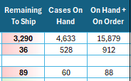
I have a pivot table where the following columns are repeated for several states, so the easiest way to create the conditional formatting would be one that works for the entire pivot table, even as states are selected and deselected and as both the columns and rows grow and shrink. I want the “On Hand + On Order” values to be highlighted when they are less than the “Remaining To Ship” value in the same row. Is it possible to use table references to these columns? If not, is there a clever / elegant way to write a single Conditional Formatting formula that would cover the entire pivot table as the table expands and contracts (both rows and columns)?
Hello! I have a pivot table where the following columns are repeated for several states, so the easiest way to create the conditional formatting would be one that works for the entire pivot table, even as states are selected and deselected and as both the columns and rows grow and shrink. I want the “On Hand + On Order” values to be highlighted when they are less than the “Remaining To Ship” value in the same row. Is it possible to use table references to these columns? If not, is there a clever / elegant way to write a single Conditional Formatting formula that would cover the entire pivot table as the table expands and contracts (both rows and columns)? Read More